For question #5 and #6, I need some guidance on how to calculate the optimal fraction of emissions control. Adding previous questions for reference.

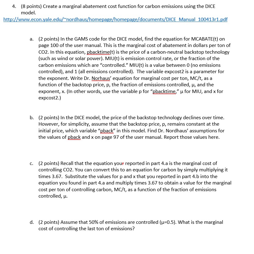
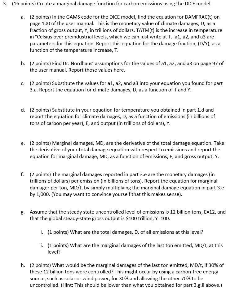
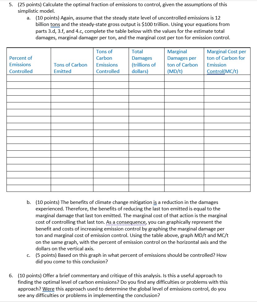
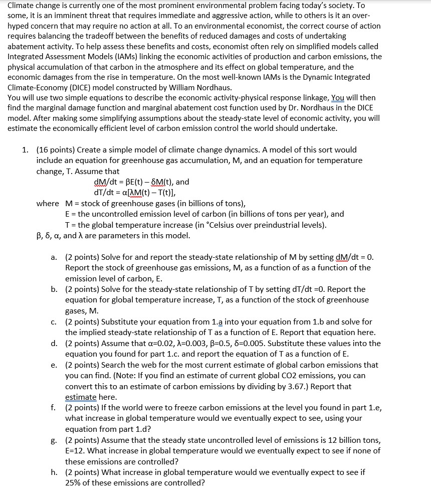
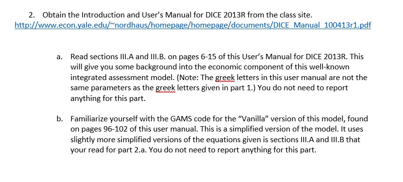
4. {8 points} Create a marginal abatement cost function for carbon emissions using the DICE model. http:www.econ.yale.eduf'\"nordhausfhomepage/homepagefdocuments/DICE Manual 100413r1.pdf a. C. (2 points] In the GAME code for the DICE modei, nd the equation for MCABATHt} on page 100 of the user manual. This is the marginal cost of abatement in dollars per ton of C02. In this equation, gbacktimeit) is the price of a carbonneutral backstop technology (such as wind or solar power). MIUIt} is emission control rate, or the fraction of the carbon emissions which are "controlled.\" MIU{t] is a value between 0 {no emissions controlled], and 1 {all emissions controlled]. The variable expoostZ is a parameter for the exponent. Write Dr. Norhaus' equation for marginal cost per ton, MCIt, as a function of the backstop price, p, the fraction of emissions controlled, p, and the exponent, x. {In other words, use the variable p for \"pbacktime,\" p for MIU, and x for expcostZ.) (2 points] In the DICE model, the price of the backstop technology declines over time. However, for simplicity, assume that the backstop price, p, remains constant at the initial price, which variable "pback" in this model. Find Dr. Nordhaus' assumptions for the values of Qback and x on page 97 of the user manual. Report those vaiues here. (2 points] Recall that the equation your reported in part 4.a is the marginal cost of controlling C02. You can convert this to an equation for carbon by simply multiplying it times 3.67. Substitute the values for p and xthat you reported in part 4.b into the equation you found in part 4.3 and multiplytimes 3.67 to obtain a value for the marginal cost per ton of controlling carbon, Mcft, as a function of the fraction of emissions controlled, p. (2 points] Assume that 50% of emissions are controlled {p205}. What is the marginal cost of controlling the last ton of emissions? Climate change is currently one of the most prominent environmental problem facing today's society. To some, it is an imminent threat that requires immediate and aggressive action, while to others is it an over- hyped concern that may require no action at all. To an environmentai economist, the correct course of action requires balancing the tradeoff between the benets of reduced damages and costs of undertaking abatement activity. To help assess these benefits and costs, economist often reiy on simplified models called Integrated Assessment Models {lAMsl linking the economic activities of production and carbon emissions, the physical accumulation of that carbon in the atmosphere and its effect on global temperature, and the economic damages from the rise in temperature. 0n the most wellknown IAMs is the Dynamic Integrated ClimateEconomy (DICE) model constructed by William Nordhaus. You will use two simple equations to describe the economic activity-physical response linkage, Q will then nd the marginal damage function and marginal abatement cost function used by Dr. Mordhaus in the DICE model. After making some simplifying assumptions about the steadystate level of economic activity, you will estimate the economically efcient ievei of carbon emission control the world should undertake. 1. {15 points} Create a simple model of climate change dynamics. A model of this sort would include an equation for greenhouse gas accumulation, M, and an equation for temperature change, 1'. Assume that mm = Eit] Mt}, and mm = aqua: To], where M 2 stock of greenhouse gases [in billions of tons), E = the uncontrolled emission level of carbon {in billions of tons per year}, and T = the giobal temperature increase (in 0Celsius over preindustrial levels}. [3, 5, u, and it are parameters in this model. a. [2 points] Solve for and report the steadystate relationship of M by setting Mdt = 0. Report the stock of greenhouse gas emissions, M, as a function of as a function of the emission level of carbon, E. b. [2 points] Solve for the steadystate relationship of T by setting dedt =0. Report the equation for global temperature increase, T, as a function of the stock of greenhouse gases, M. c. (2 points] Substitute your equation from Lg into your equation from 1.b and solve for the implied steadystate relationship of T as a function of E. Report that equation here. d. (2 points] Assume that o=D.02, "#0303, B=G.5, 6:0.005. Substitute these values into the equation you found for part Lo. and report the equation of T as a function of E. e. (2 points] Search the web for the most current estimate of global carbon emissions that you can find. [Note: If you find an estimate of current global CO2 emissions, you can convert this to an estimate of carbon emissions by dividing by 3.67.} Report that estimate here. f. (2 points] If the world were to freeze carbon emissions at the ievel you found in part Le, what increase in global temperature would we eventually expect to see, using your equation from part 1.d? g. (2 points] Assume that the steady state uncontrolled level of emissions is 12 billion tons, E=12. What increase in global temperature would we eventually expect to see if none of these emissions are controlled? h. (2 points] What increase in global temperature wouid we eventually expect to see if 25% of these emissions are controlled? 2. l[llbtain the Introduction and User's Manual for DICE 2013B from the class site. htt : www.econ. ale.edu "nordhaus ome e home a e documents DICE Manual 100413r1. df a. Read sections "LA and \"LE. on pages 615 of this User's Manual for DICE 2013R. This will give 'you some background into the economic component of this wellknown integrated assessment model. (Note: The Egg; letters in this user manual are not the same parameters as the gLeneh letters given in part 1.} You do not need to report anything for this part. b. Familiarize yourself with the GAMS code for the \"Vanilla\" version of this model, found on pages 9&102 of this user manual. This is a simplified version of the model. It uses slightiv more simplied versions of the equations given is sections "LA and "LB that your read for part 2.a. You do not need to report anything for this part. 3. {16 points} Create a marginal damage function for carbon emissions using the DICE model. a. (2 points} In the GAMS code for the DICE model, nd the equation for DAMFRACH] on page 100 of the user manual. This is the monetary value of climate damages, D, as a fraction of gross output, Y, in trillions of dollars. TATMlt] is the increase in temperature in \"Celsius over preindustrial levels, which we can just write at T. a1, a2, and 33 are parameters for this equation. Report this equation for the damage fraction, {DH}, as a function of the temperature increase, T. b. [2 points] Find Dr. Nordhaus' assumptions for the values of a1, 32, and a3 on page 97 of the user manual. Report those values here. c. [2 points] Substitute the values for al, a2, and a3 into your equation you found for past 3.a. Report the equation for climate damages, D, as a function ofT and Y. d. (2 points] Substitute in your equation for temperature you obtained in part 1.d and repmt the equation for ciimate damages, D, as a function of emissions [in billions of tons of carbon per year], E, and output (in trillions of dollars], Y. e. (2 points] Marginal damages, MD, are the derivative of the total damage equation. Take the derivative of your total damage equation with respect to emissions and report the equation for marginal damage, MD, as a function of emissions, E, and gross output, Y. f. (2 points] The marginal damages reported in part 3.e are the monetary damages [in trillions of dollars} per emission {in biliions of tons]. Report the equation for marginal damager per ton, MD,-"t, by simply muttiplying the marginal damage equation in part 3.e by 1,000. {You may want to convince yourself that this makes sense}. g. Assume that the steady state uncontrolled level of emissions is 12 billion tons, E212, and that the global steadystate gross output is $100 trillion, Y=100. i. {1 points) What are the total damages, D, of all emissions at this level? ii. {1 points) What are the marginal damages of the last ton emitted, Mth, at this level? h. (2 points] What would be the marginal damages of the last ton emitted, Mth, if 30% of these 12 billion tons were controlled? This might occur by using a carbonfree energy source, such as solar or wind power, for 30% and allowing the other ?0% to be uncontrolled. (Hint: This should be lower than what you obtained for part 3.g.ii above} 5. (25 points) Calculate the optimal fraction of emissions to control, given the assumptions of this simplistic model. a. (10 points) Again, assume that the steady state level of uncontrolled emissions is 12 billion tons and the steady-state gross output is $100 trillion. Using your equations from parts 3.d, 3.f, and 4.c, complete the table below with the values for the estimate total damages, marginal damager per ton, and the marginal cost per ton for emission control. Tons of Total Marginal Marginal Cost per Percent of Carbon Damages Damages per ton of Carbon for Emissions Tons of Carbon Emissions (trillions of ton of Carbon Emission Controlled Emitted Controlled dollars (MD/t) Control(MC/t) b. (10 points) The benefits of climate change mitigation is a reduction in the damages experienced. Therefore, the benefits of reducing the last ton emitted is equal to the marginal damage that last ton emitted. The marginal cost of that action is the marginal cost of controlling that last ton. As a consequence, you can graphically represent the benefit and costs of increasing emission control by graphing the marginal damage per ton and marginal cost of emission control. Using the table above, graph MD/t and MC/t on the same graph, with the percent of emission control on the horizontal axis and the dollars on the vertical axis. c. (5 points) Based on this graph in what percent of emissions should be controlled? How did you come to this conclusion? 6. (10 points) Offer a brief commentary and critique of this analysis. Is this a useful approach to finding the optimal level of carbon emissions? Do you find any difficulties or problems with this approach? Were this approach used to determine the global level of emissions control, do you see any difficulties or problems in implementing the conclusion