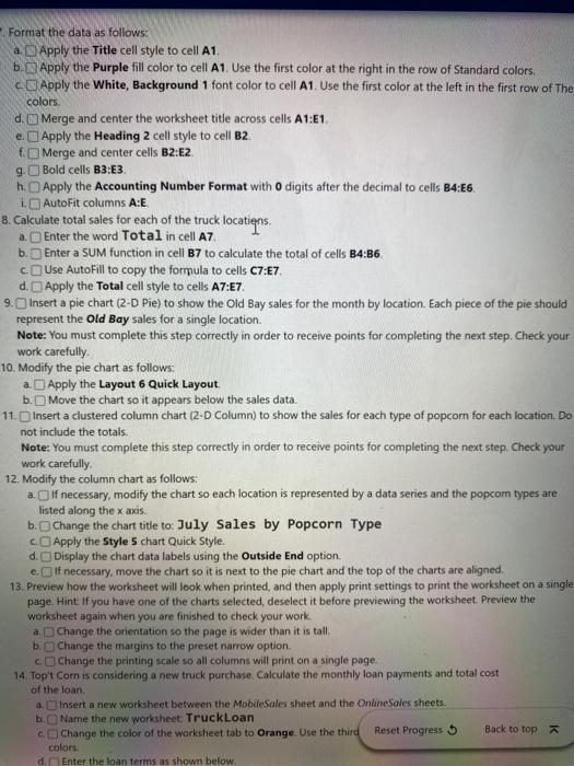
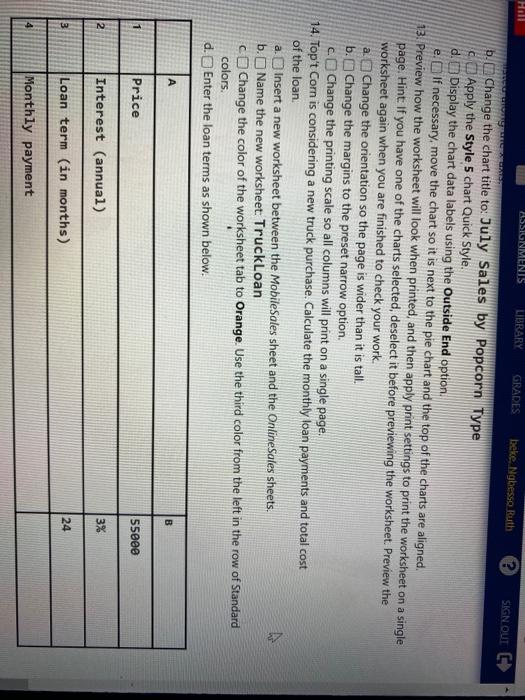
Format the data as follows: a. Apply the Title cell style to cell A1. b. Apply the Purple fill color to cell A1. Use the first color at the right in the row of Standard colors. c)Apply the White Background 1 font color to cell A1. Use the first color at the left in the first row of The colors d. Merge and center the worksheet title across cells A1:51 e Apply the Heading 2 cell style to cell B2. Merge and center cells B2:E2 g. Bold cells B3:53 h. Apply the Accounting Number Format with o digits after the decimal to cells B4:E6. 1.AutoFit columns A:E 8. Calculate total sales for each of the truck locatiens a. Enter the word Total in cell A7 b. Enter a SUM function in cell B7 to calculate the total of cells B4:36 cUse AutoFill to copy the formula to cells C7:E7 d. Apply the Total cell style to cells A7:07 9. Insert a pie chart (2-D Pie) to show the Old Bay sales for the month by location. Each piece of the pie should represent the Old Bay sales for a single location. Note: You must complete this step correctly in order to receive points for completing the next step. Check your work carefully 10. Modify the pie chart as follows: a. Apply the Layout 6 Quick Layout b. Move the chart so it appears below the sales data. 11. Insert a clustered column chart (2-D Column) to show the sales for each type of popcorn for each location. Do not include the totals Note: You must complete this step correctly in order to receive points for completing the next step. Check your work carefully 12. Modify the column chart as follows: a. C) If necessary, modify the chart so each location is represented by a data series and the popcorn types are listed along the x axis b. Change the chart title to: July Sales by Popcorn Type Apply the Style 5 chart Quick Style. d. Display the chart data labels using the Outside End option e if necessary, move the chart so it is next to the pie chart and the top of the charts are aligned. 13. Preview how the worksheet will look when printed, and then apply print settings to print the worksheet on a single page. Hint: If you have one of the charts selected, deselect it before previewing the worksheet Preview the worksheet again when you are finished to check your work a. Change the orientation so the page is wider than it is tall. b. Change the margins to the preset narrow option Change the printing scale so all columns will print on a single page 14. Top't Com is considering a new truck purchase. Calculate the monthly loan payments and total cost a. Insert a new worksheet between the MobileSales sheet and the Online Sales sheets. b. Name the new worksheet TruckLoan c. Change the color of the worksheet tab to Orange. Use the third Reset Progress 3 Back to top of the loan colors a Enter the loan terms as shown below. Hill ASSIGNMENIS GRADES LIBRARY beke Nabesso Ruth ? SIGN OUT C b. Change the chart title to: July Sales by Popcorn Type Apply the Style 5 chart Quick Style. d. 1 Display the chart data labels using the Outside End option. e. If necessary, move the chart so it is next to the pie chart and the top of the charts are aligned. 13. Preview how the worksheet will look when printed, and then apply print settings to print the worksheet on a single page. Hint If you have one of the charts selected, deselect it before previewing the worksheet. Preview the worksheet again when you are finished to check your work. a Change the orientation so the page is wider than it is tall. b. Change the margins to the preset narrow option cChange the printing scale so all columns will print on a single page. 14. Top't Corn is considering a new truck purchase. Calculate the monthly loan payments and total cost of the loan. a. Insert a new worksheet between the MobileSales sheet and the Online Sales sheets. b.Name the new worksheet: TruckLoan cChange the color of the worksheet tab to Orange. Use the third color from the left in the row of Standard colors d. Enter the loan terms as shown below. B 1 Price 55000 2 Interest (annual) 3% 3 Loan term (in months) 24 4 Monthly payment Format the data as follows: a. Apply the Title cell style to cell A1. b. Apply the Purple fill color to cell A1. Use the first color at the right in the row of Standard colors. c)Apply the White Background 1 font color to cell A1. Use the first color at the left in the first row of The colors d. Merge and center the worksheet title across cells A1:51 e Apply the Heading 2 cell style to cell B2. Merge and center cells B2:E2 g. Bold cells B3:53 h. Apply the Accounting Number Format with o digits after the decimal to cells B4:E6. 1.AutoFit columns A:E 8. Calculate total sales for each of the truck locatiens a. Enter the word Total in cell A7 b. Enter a SUM function in cell B7 to calculate the total of cells B4:36 cUse AutoFill to copy the formula to cells C7:E7 d. Apply the Total cell style to cells A7:07 9. Insert a pie chart (2-D Pie) to show the Old Bay sales for the month by location. Each piece of the pie should represent the Old Bay sales for a single location. Note: You must complete this step correctly in order to receive points for completing the next step. Check your work carefully 10. Modify the pie chart as follows: a. Apply the Layout 6 Quick Layout b. Move the chart so it appears below the sales data. 11. Insert a clustered column chart (2-D Column) to show the sales for each type of popcorn for each location. Do not include the totals Note: You must complete this step correctly in order to receive points for completing the next step. Check your work carefully 12. Modify the column chart as follows: a. C) If necessary, modify the chart so each location is represented by a data series and the popcorn types are listed along the x axis b. Change the chart title to: July Sales by Popcorn Type Apply the Style 5 chart Quick Style. d. Display the chart data labels using the Outside End option e if necessary, move the chart so it is next to the pie chart and the top of the charts are aligned. 13. Preview how the worksheet will look when printed, and then apply print settings to print the worksheet on a single page. Hint: If you have one of the charts selected, deselect it before previewing the worksheet Preview the worksheet again when you are finished to check your work a. Change the orientation so the page is wider than it is tall. b. Change the margins to the preset narrow option Change the printing scale so all columns will print on a single page 14. Top't Com is considering a new truck purchase. Calculate the monthly loan payments and total cost a. Insert a new worksheet between the MobileSales sheet and the Online Sales sheets. b. Name the new worksheet TruckLoan c. Change the color of the worksheet tab to Orange. Use the third Reset Progress 3 Back to top of the loan colors a Enter the loan terms as shown below. Hill ASSIGNMENIS GRADES LIBRARY beke Nabesso Ruth ? SIGN OUT C b. Change the chart title to: July Sales by Popcorn Type Apply the Style 5 chart Quick Style. d. 1 Display the chart data labels using the Outside End option. e. If necessary, move the chart so it is next to the pie chart and the top of the charts are aligned. 13. Preview how the worksheet will look when printed, and then apply print settings to print the worksheet on a single page. Hint If you have one of the charts selected, deselect it before previewing the worksheet. Preview the worksheet again when you are finished to check your work. a Change the orientation so the page is wider than it is tall. b. Change the margins to the preset narrow option cChange the printing scale so all columns will print on a single page. 14. Top't Corn is considering a new truck purchase. Calculate the monthly loan payments and total cost of the loan. a. Insert a new worksheet between the MobileSales sheet and the Online Sales sheets. b.Name the new worksheet: TruckLoan cChange the color of the worksheet tab to Orange. Use the third color from the left in the row of Standard colors d. Enter the loan terms as shown below. B 1 Price 55000 2 Interest (annual) 3% 3 Loan term (in months) 24 4 Monthly payment


