Question
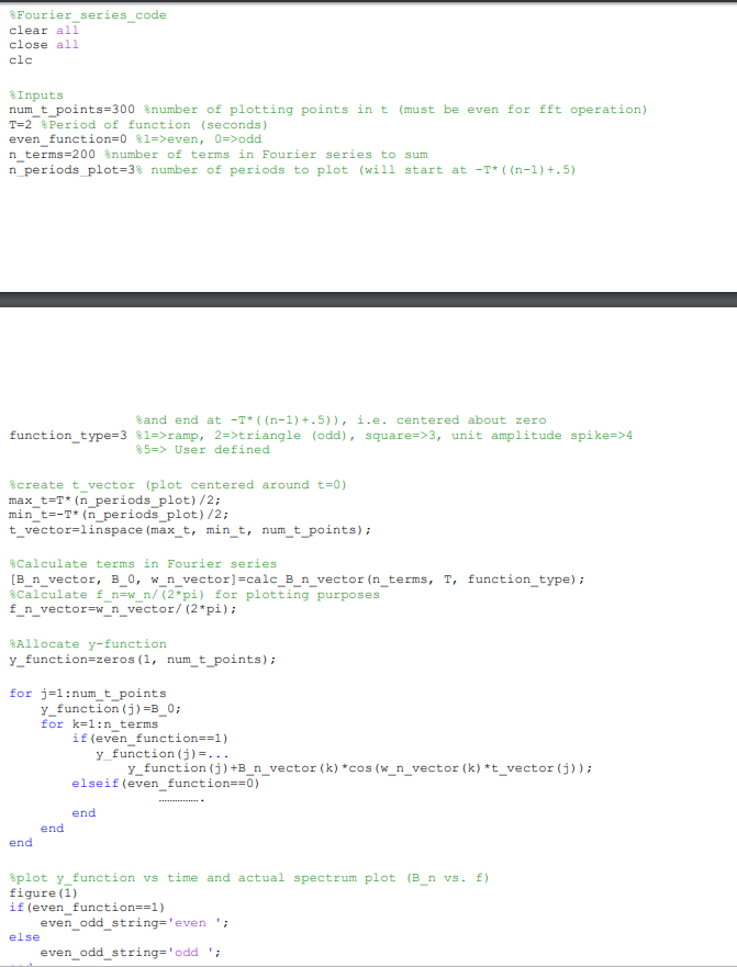
%Fourier_series_code clear all close all clc %Inputs num_t_points=300 %number of plotting points in t (must be even for fft operation) T=2 %Period of function (seconds)


%Fourier_series_code clear all close all clc %Inputs num_t_points=300 %number of plotting points in t (must be even for fft operation) T=2 %Period of function (seconds) even_function=0 %1=>even, 0=>odd n_terms=200 %number of terms in Fourier series to sum n_periods_plot=3% number of periods to plot (will start at -T*((n-1)+.5) %and end at -T*((n-1)+.5)), i.e. centered about zero function_type=3 %1=>ramp, 2=>triangle (odd), square=>3, unit amplitude spike=>4 %5=> User defined
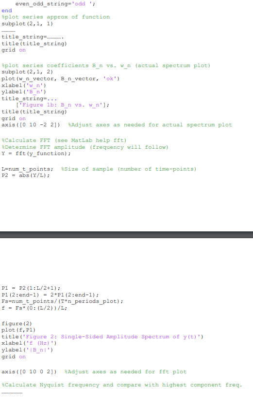
%create t_vector (plot centered around t=0) max_t=T*(n_periods_plot)/2; min_t=-T*(n_periods_plot)/2; t_vector=linspace(max_t, min_t, num_t_points); %Calculate terms in Fourier series [B_n_vector, B_0, w_n_vector]=calc_B_n_vector(n_terms, T, function_type); %Calculate f_n=w_n/(2*pi) for plotting purposes f_n_vector=w_n_vector/(2*pi); %Allocate y-function y_function=zeros(1, num_t_points); for j=1:num_t_points y_function(j)=B_0; for k=1:n_terms if(even_function==1) y_function(j)=... y_function(j)+B_n_vector(k)*cos(w_n_vector(k)*t_vector(j)); elseif(even_function==0) . end end end %plot y_function vs time and actual spectrum plot (B_n vs. f) figure(1) if(even_function==1) even_odd_string='even '; else even_odd_string='odd '; end %plot series approx of function subplot(2,1, 1) title_string=. title(title_string) grid on %plot series coefficients B_n vs. w_n (actual spectrum plot) subplot(2,1, 2) plot(w_n_vector, B_n_vector, 'ok') xlabel('w_n') ylabel('B_n') title_string=... ['Figure 1b: B_n vs. w_n']; title(title_string) grid on axis([0 10 -2 2]) %Adjust axes as needed for actual spectrum plot %Calculate FFT (see MatLab help fft) %Determine FFT amplitude (frequency will follow) Y = fft(y_function); L=num_t_points; %Size of sample (number of time-points) P2 = abs(Y/L); P1 = P2(1:L/2+1); P1(2:end-1) = 2*P1(2:end-1); Fs=num_t_points/(T*n_periods_plot); f = Fs*(0:(L/2))/L; figure(2) plot(f,P1) title('Figure 2: Single-Sided Amplitude Spectrum of y(t)') xlabel('f (Hz)') ylabel('|B_n|') grid on axis([0 10 0 2]) %Adjust axes as needed for fft plot %Calculate Nyquist frequency and compare with highest component freq.
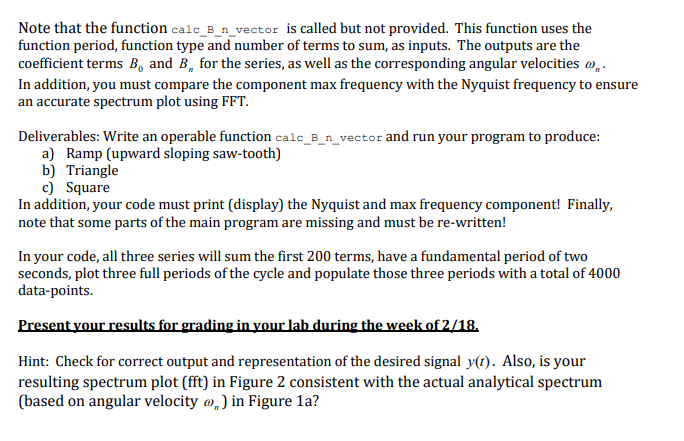
Matlab Component You are provided with a fragment of a MatLab code which calculates and plots a Fourier series y(1)-Bo + B" cos(o,1) or y(1)-B + B, sin (a,1). The code plots a "ramp", "triangle" and "square" periodic function with period T. The code requires inputs such as the number of terms N to sum in the series and the number of periods to plot. In addition, the code can sum an even or odd series as specified The main code is given below: %Fourier series code clear all close all clc %Inputs num-t-points-300 %number of plotting points in t (must be even for fft operation) T=2 %Period of function (seconds ) even function=0 81=>even, 0=>odd nterms =200 %number of terms in Fourier series to sum n-periods plot-3% number of periods to plot (will start at -me ((n-11+.5) - and end at -T(n-1) +.5)), i.e. centered about zero function-type-3 %1 %5=> 2 defined triangle (odd), squares) 3, unit amplitude spikes)4 ramp, User screate t_vector (plot centered around t-0) max t-T*(n periods plot)/2 min-t-T* (n-periods-plot) /2; t_vector-linspace (max t, min t, num t points) %Calculate terms in Fourier series B_n_vector, B0, w n vector]-calc_B_n_vector (n_terms, T. function type) Calculate f-nwn/ (2*pi) for plotting purposes f-n-vector n-vector/ (2*pi) ; %Allocate y-function y function-zeros(1, num_t_points) for i=1 : num t points y function (j)-B0; for k=1:n terms if (even function==1) y function ()-.. y function (j)+Bn_vector (k) cos (w n vector (k) *t_vector (j)) elseif (even function==0) end end end %plot y-function vs time and actual spectrum plot figure (1) if (even function==1) (B-n vs. f) even_ odd string-even 'i else even_ odd string-'odd even_odd string-odd'i end %plot series approx of function subplot (2,1, 1) title_string. title (title _string) grid on %plot series coefficients B-n vs. wn (actual spectrum plot) subplot (2,1, 2) plot (w nvector, B n vector, 'ok') xlabel ('wn') ylabel ('Bn' title string-... 'Figure 1b: Bn vs. w n' title (title _string) grid on axis (0 10 -2 2]) Adjust axes as needed for actual spectrum plot Calculate FFT (see MatLab help fft) Determine FFT amplitude (frequency will follow) Y fft (y-function); 1-num-t-points ; P2 = abs (Y/L) ; %Size of sample (number of time-points) P1P2 (1:L/2+1) P1 (2:end-1)2*P1 (2:end-1) s-num t points/(T"n periods plot) fs(0: (L/2))/L figure (2) plot (f, P1) title('Figure 2: Single-sided Amplitude Spectrum of y(t) xlabel(' (Hz)' ylabel ('IB nl' grid on axis([0 10 0 2]) %Adjust axes as needed for fft plot Calculate Nyquist frequency and compare with highest component freq Note that the function calc_B_n_vector is called but not provided. This function uses the function period, function type and number of terms to sum, as inputs. The outputs are the coefficient terms B, and B, for the series, as well as the corresponding angular velocities In addition, you must compare the component max frequency with the Nyquist frequency to ensure an accurate spectrum plot using FFT Deliverables: Write an operable function calc_Bn_vector and run your program to produce: a) Ramp (upward sloping saw-tooth) b) Triangle c) Square In addition, your code must print (display) the Nyquist and max frequency component! Finally, note that some parts of the main program are missing and must be re-written! In your code, all three series will sum the first 200 terms, have a fundamental period of two seconds, plot three full periods of the cycle and populate those three periods with a total of 4000 data-points. Present your results for grading in your lab during the week of2/18. Hint: Check for correct output and representation of the desired signal y(t). Also, is your resulting spectrum plot (fft) in Figure 2 consistent with the actual analytical spectrum (based on angular velocity o) in Figure 1a? Matlab Component You are provided with a fragment of a MatLab code which calculates and plots a Fourier series y(1)-Bo + B" cos(o,1) or y(1)-B + B, sin (a,1). The code plots a "ramp", "triangle" and "square" periodic function with period T. The code requires inputs such as the number of terms N to sum in the series and the number of periods to plot. In addition, the code can sum an even or odd series as specified The main code is given below: %Fourier series code clear all close all clc %Inputs num-t-points-300 %number of plotting points in t (must be even for fft operation) T=2 %Period of function (seconds ) even function=0 81=>even, 0=>odd nterms =200 %number of terms in Fourier series to sum n-periods plot-3% number of periods to plot (will start at -me ((n-11+.5) - and end at -T(n-1) +.5)), i.e. centered about zero function-type-3 %1 %5=> 2 defined triangle (odd), squares) 3, unit amplitude spikes)4 ramp, User screate t_vector (plot centered around t-0) max t-T*(n periods plot)/2 min-t-T* (n-periods-plot) /2; t_vector-linspace (max t, min t, num t points) %Calculate terms in Fourier series B_n_vector, B0, w n vector]-calc_B_n_vector (n_terms, T. function type) Calculate f-nwn/ (2*pi) for plotting purposes f-n-vector n-vector/ (2*pi) ; %Allocate y-function y function-zeros(1, num_t_points) for i=1 : num t points y function (j)-B0; for k=1:n terms if (even function==1) y function ()-.. y function (j)+Bn_vector (k) cos (w n vector (k) *t_vector (j)) elseif (even function==0) end end end %plot y-function vs time and actual spectrum plot figure (1) if (even function==1) (B-n vs. f) even_ odd string-even 'i else even_ odd string-'odd even_odd string-odd'i end %plot series approx of function subplot (2,1, 1) title_string. title (title _string) grid on %plot series coefficients B-n vs. wn (actual spectrum plot) subplot (2,1, 2) plot (w nvector, B n vector, 'ok') xlabel ('wn') ylabel ('Bn' title string-... 'Figure 1b: Bn vs. w n' title (title _string) grid on axis (0 10 -2 2]) Adjust axes as needed for actual spectrum plot Calculate FFT (see MatLab help fft) Determine FFT amplitude (frequency will follow) Y fft (y-function); 1-num-t-points ; P2 = abs (Y/L) ; %Size of sample (number of time-points) P1P2 (1:L/2+1) P1 (2:end-1)2*P1 (2:end-1) s-num t points/(T"n periods plot) fs(0: (L/2))/L figure (2) plot (f, P1) title('Figure 2: Single-sided Amplitude Spectrum of y(t) xlabel(' (Hz)' ylabel ('IB nl' grid on axis([0 10 0 2]) %Adjust axes as needed for fft plot Calculate Nyquist frequency and compare with highest component freq Note that the function calc_B_n_vector is called but not provided. This function uses the function period, function type and number of terms to sum, as inputs. The outputs are the coefficient terms B, and B, for the series, as well as the corresponding angular velocities In addition, you must compare the component max frequency with the Nyquist frequency to ensure an accurate spectrum plot using FFT Deliverables: Write an operable function calc_Bn_vector and run your program to produce: a) Ramp (upward sloping saw-tooth) b) Triangle c) Square In addition, your code must print (display) the Nyquist and max frequency component! Finally, note that some parts of the main program are missing and must be re-written! In your code, all three series will sum the first 200 terms, have a fundamental period of two seconds, plot three full periods of the cycle and populate those three periods with a total of 4000 data-points. Present your results for grading in your lab during the week of2/18. Hint: Check for correct output and representation of the desired signal y(t). Also, is your resulting spectrum plot (fft) in Figure 2 consistent with the actual analytical spectrum (based on angular velocity o) in Figure 1aStep by Step Solution
There are 3 Steps involved in it
Step: 1

Get Instant Access to Expert-Tailored Solutions
See step-by-step solutions with expert insights and AI powered tools for academic success
Step: 2

Step: 3

Ace Your Homework with AI
Get the answers you need in no time with our AI-driven, step-by-step assistance
Get Started


