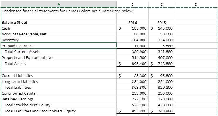
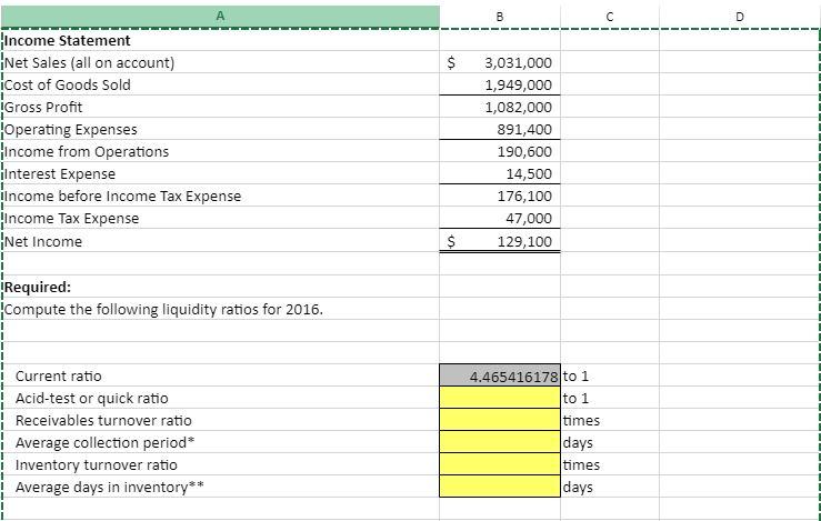
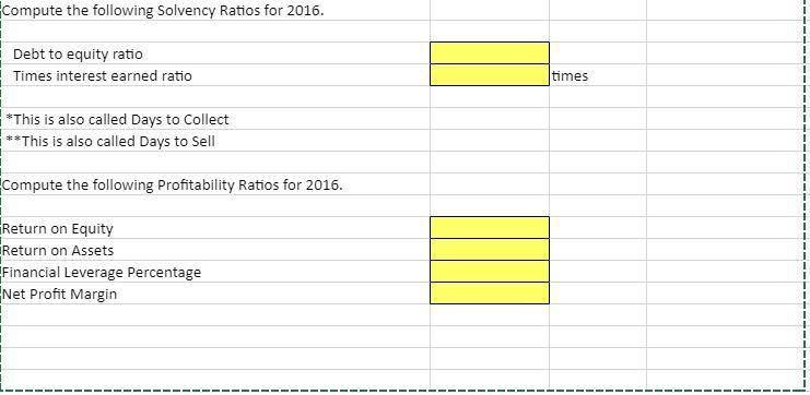
Games Galore has summarized its condensed financial statements for the past two years. The Controller has asked you to compute the liquidity, solvency and profitability ratios for 2016. Use the information included in the Excel Simulation and the Excel functions described below to complete the task. Be sure to use 365 days in a year where necessary. Cell Reference: Allows you to refer to data from another cell in the worksheet. From the Excel Simulation below, if in a blank cell, =C6 was entered, the formula would output the result from cell C6, or 134,000 in this example. Basic Math functions: Allows you to use the basic math symbols to perform mathematical functions. You can use the following keys: + (plus sign to add), - (minus sign to subtract), * (asterisk sign to multiply), and / (forward slash to divide). From the Excel Simulation below, if in a blank cell =B8+B9 was entered, the formula would add the values from those cells and output the result, or 895,400 in this example. If using the other math symbols the result would output an appropriate answer for its function. SUM function: Allows you to refer to multiple cells and adds all the values. You can add individual cell references or ranges to utilize this function. From the Excel Simulation below, if in a blank cell =SUM(C4,C5,C6) was entered, the formula would output the result of adding those three separate cells, or 336,000 in this example. Similarly, if in a blank cell =SUM(C4:C6) was entered, the formula would output the same result of adding those cells, except they are expressed as a range in the formula, and the result would be 336,000 in this example. AVERAGE function: Allows you to average any number of cells included in the formula. The syntax of the AVERAGE function is =AVERAGE(number1,number2,) and returns the result of the mathematical calculation for the average of the arguments included in the formula. The arguments of number1 and number2 can be a numeric value or a cell reference. From the Excel Simulation below, if in a blank cell =AVERAGE(B4,B5,C4,C5) was entered, the formula would output the result of averaging these four cells, or 116,750 in this example.

Games Galore has summarized its condensed financial statements for the past two years. The Controller has asked you to compute the liquidity, solvency and profitability ratios for 2016. Use the information included in the Excel Simulation and the Excel functions described below to complete the task. Be sure to use 365 days in a year where necessary.

• Cell Reference: Allows you to refer to data from another cell in the worksheet. From the Excel Simulation below, if in a blank cell, =C6 was entered, the formula would output the result from cell C6, or 134,000 in this example.
• Basic Math functions: Allows you to use the basic math symbols to perform mathematical functions. You can use the following keys: + (plus sign to add), - (minus sign to subtract), * (asterisk sign to multiply), and / (forward slash to divide). From the Excel Simulation below, if in a blank cell =B8+B9 was entered, the formula would add the values from those cells and output the result, or 895,400 in this example. If using the other math symbols the result would output an appropriate answer for its function.
• SUM function: Allows you to refer to multiple cells and adds all the values. You can add individual cell references or ranges to utilize this function. From the Excel Simulation below, if in a blank cell =SUM(C4,C5,C6) was entered, the formula would output the result of adding those three separate cells, or 336,000 in this example. Similarly, if in a blank cell =SUM(C4:C6) was entered, the formula would output the same result of adding those cells, except they are expressed as a range in the formula, and the result would be 336,000 in this example.
• AVERAGE function: Allows you to average any number of cells included in the formula. The syntax of the AVERAGE function is =AVERAGE(number1,number2,) and returns the result of the mathematical calculation for the average of the arguments included in the formula. The arguments of number1 and number2 can be a numeric value or a cell reference. From the Excel Simulation below, if in a blank cell =AVERAGE(B4,B5,C4,C5) was entered, the formula would output the result of averaging these four cells, or 116,750 in this example.

B D Condensed financial statements for Games Galore are summarized below: 1 1 $ Balance Sheet Cash Accounts Receivable, Net Inventory Prepaid Insurance Total Current Assets Property and Equipment, Net Total Assets 2016 2015 185,000 $ 143,000 80,000 59,000 104,000 134,000 11,900 5,880 380,900 341,880 514,500 407,000 895,400 $ 748,880 $ $ Current Liabilities Long-term Liabilities Total Liabilities Contributed Capital Retained Earnings Total Stockholders' Equity Total Liabilities and Stockholders' Equity 85,300 $ 96,800 284,000 224,000 369,300 320,800 299,000 299,000 227,100 129,080 526,100 428,080 895,400 $ 748,880 $ B C $ Income Statement Net Sales (all on account) Cost of Goods Sold Gross Profit Operating Expenses Income from Operations Interest Expense Income before Income Tax Expense Income Tax Expense Net Income 1 Required: Compute the following liquidity ratios for 2016. 3,031,000 1,949,000 1,082,000 891,400 190,600 14,500 176,100 47,000 129,100 $ 1 I 1 Current ratio Acid-test or quick ratio Receivables turnover ratio Average collection period Inventory turnover ratio Average days in inventory** 4.465416178 to 1 to 1 times days times days . Compute the following Solvency Ratios for 2016. Debt to equity ratio Times interest earned ratio times *This is also called Days to Collect **This is also called Days to Sell 1 1 Compute the following Profitability Ratios for 2016. Return on Equity Return on Assets Financial Leverage Percentage Net Profit Margin 1