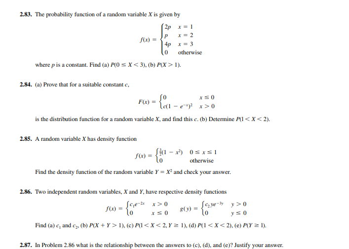
GIVE DETAILED WORKING IN ALL QUESTIONS.

Suppose that a game is to be played with a single die assumed fair. In this game a player wins $20 if a 2 turns up, $40 if a 4 turns up; loses $30 if a 6 turns up; while the player neither wins nor loses if any other face turns up. Find the expected sum of money to be won

The average travel time to a distant city is c hours by car or b hours by bus. A woman cannot decide whether to drive or take the bus, so she tosses a coin. What is her expected travel time?

1. In a lottery there are 200 prizes of $5, 20 prizes of $25, and 5 prizes of $100. Assuming that 10,000 tickets are to be issued and sold, what is a fair price to pay for a ticket?

3.36. Determine, (a) the semi-interquartile range, (b) the mean deviation for the distribution of Problem 3.33.

3.39. Let X be a random variable that takes on the values xk k with probabilities pk where k 1, . . . , n. (a) Find the characteristic function ( ) of X, (b) obtain pk in terms of (X)

The values of a standardized variable are sometimes called standard scores, and X is then said to be expressed in standard units (i.e., is taken as the unit in measuring X - ). Standardized variables are useful for comparing different distributions.

Generalizations of Theorem 3-9 to more than two independent random variables are easily made. In words, the moment generating function of a sum of independent random variables is equal to the product of their moment generating functions

An important reason for introducing the characteristic function is that (37) represents the Fourier transform of the density function f(x). From the theory of Fourier transforms, we can easily determine the density function from the characteristic function. In fact, (42) which is often called an inversion formula, or inverse Fourier transform. In a similar manner we can show in the discrete case that the probability function f(x) can be obtained from (36) by use of Fourier series, which is the analog of the Fourier integral for the discrete case. See Problem 3.39. Another reason for using the characteristic function is that it always exists whereas the moment generating function may not exist

the probability of X differing from its mean by more than 2 standard deviations is less than or equal to 0.25; equivalently, the probability that X will lie within 2 standard deviations of its mean is greater than or equal to 0.75. This is quite remarkable in view of the fact that we have not even specified the probability distribution of X

1. MODE. The mode of a discrete random variable is that value which occurs most often or, in other words, has the greatest probability of occurring. Sometimes we have two, three, or more values that have relatively large probabilities of occurrence. In such cases, we say that the distribution is bimodal, trimodal, or multimodal, respectively. The mode of a continuous random variable X is the value (or values) of X where the probability density function has a relative maximum. 2. MEDIAN. The median is that value x for which and P(X x) In the case of a continuous distribution we have and the median separates the density curve into two parts having equal areas of 1 2 each. In the case of a discrete distribution a unique median may not exist

3.34. A discrete random variable has probability function f(x) 1 2x where x 1, 2, . . . . Find (a) the mode, (b) the median, and (c) compare them with the mean. (a) The mode is the value x having largest associated probability. In this case it is x 1, for which the probability is 1 2. (b) If x is any value between 1 and 2, and Therefore, any number between 1 and 2 could represent the median. For convenience, we choose the midpoint of the interval, i.e., 3 2. (c) As found in Problem 3.3,

3.65. Find the first four moments about the mean in (a) Problem 3.43, (b) Problem 3.44. 3.66. (a) Find the moment generating function of a random variable having density function and (b) determine the first four moments about the origin. 3.67. In Problem 3.66 find the first four moments about the mean. 3.68. Let X have density function . Find the kth moment about (a) the origin, (b) the mean. 3.69. If M(t) is the moment generating function of the random variable X, prove that the 3rd and 4th moments about

Discrete distribution functions 2.43. The probability function of a random variable X is shown in Table 2-7. Construct a table giving the distribution function of X. Table 2-7 Table 2-8 2 3 X 1 2 3 4 f(x) 1/2 1/3 1/6 F(x) 1/8 3/8 3/4 2.44. Obtain the distribution function for (a) Problem 2.38, (b) Problem 2.39, (c) Problem 2.40. 2.45. Obtain the distribution function for (a) Problem 2.41, (b) Problem 2.42. 2.46. Table 2-8 shows the distribution function of a random variable X. Determine (a) the probability function, (b) P(1 = X = 3), (c) P(X = 2). (d) P(X 1.4). Continuous random variables and probability distributions 2.47. A random variable X has density function f (x) = [ce- 3 x30 Find (a) the constant c, (b) P(1 1), (d) P(1 1), (d) the distribution function. Joint distributions and independent variables 2.54. The joint probability function of two discrete random variables X and Y is given by f(x, y) = cry for x = 1, 2, 3 and y = 1, 2, 3, and equals zero otherwise. Find (a) the constant c, (b) P(X - 2. Y = 3), (c) P(1 = X = 2, Y = 2), (d) P(X = 2), (e) P(Y 1). 2.84. (a) Prove that for a suitable constant c, F(x) = Icd - ex x30 is the distribution function for a random variable X, and find this c. (b) Determine (1 1), (c) P(1