:::Give step by step solutions.

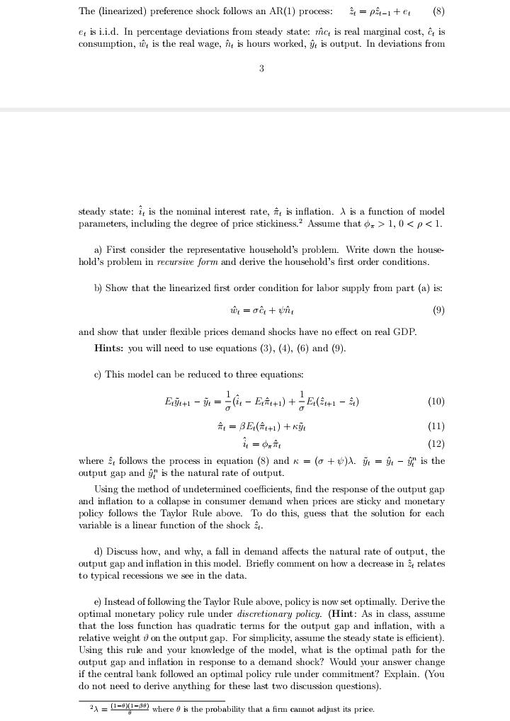
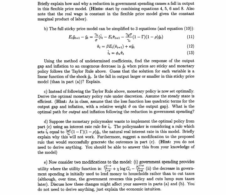
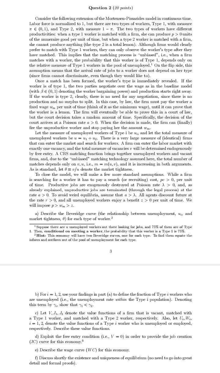
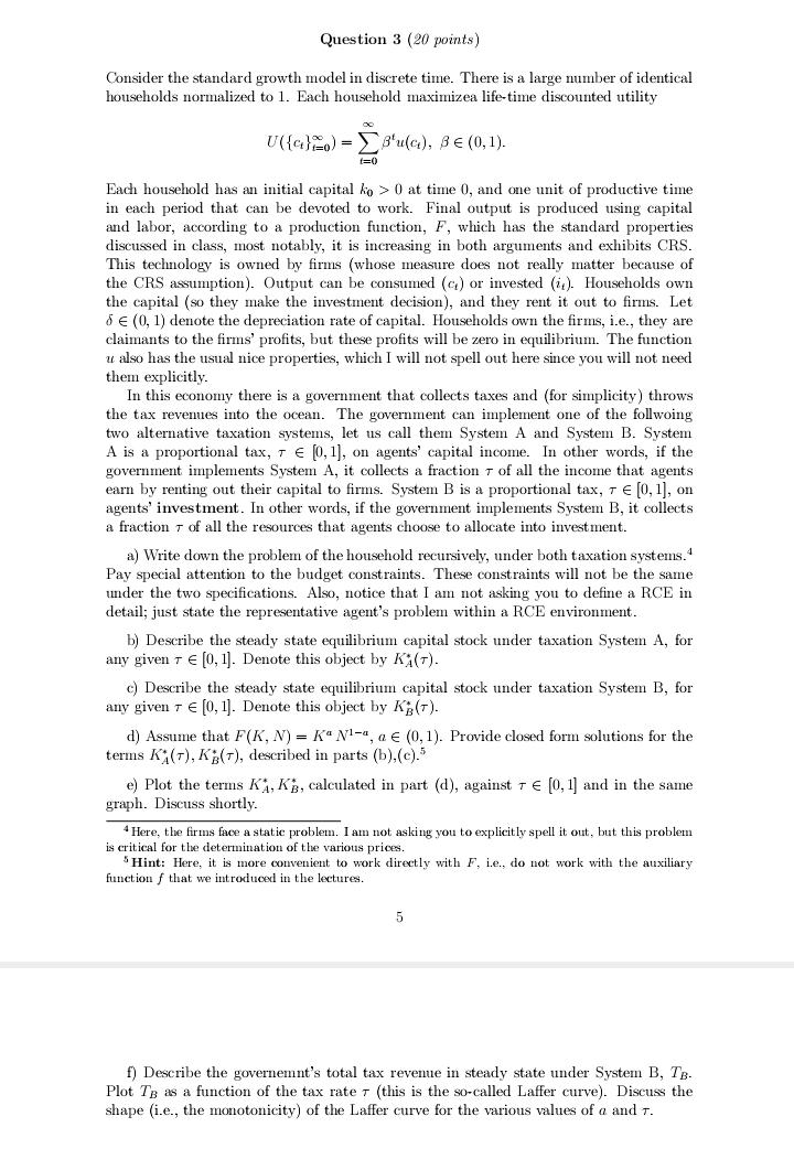
The (linearized) preference shock follows an AR(1) process: & = pa-1 + er (8) er is i.i.d. In percentage deviations from steady state: me, is real marginal cost, & is consumption, w, is the real wage, f is hours worked, y, is output. In deviations from 3 steady state: i, is the nominal interest rate, #, is inflation. A is a function of model parameters, including the degree of price stickiness." Assume that o. > 1, 0 O units of the numeraire good per unit of time, but when a type 2 worker is matched with a firm, she cannot produce anything (the type 2 is a total lemon). Although firms would clearly prefer to match with Type 1 workers, they can only observe the worker's type after they have matched. This implies that the matching process is "unbiased", i.e., when a firm matches with a worker, the probability that this worker is of Type 1, depends only on the relative measure of Type 1 workers in the pool of unemployed.' On the flip side, this assumption means that the arrival rate of jobs to a worker does not depend on her type (since firms cannot discriminate, even though they would like to). Once a match has been formed, the worker's type is immediately revealed. If the worker is of type 1, the two parties negotiate over the wage as in the baseline model (with B E (0, 1) denoting the worker bargaining power) and production starts right away. If the worker is type 2, clearly, there is no need for any negotiation, since there is no production and no surplus to split. In this case, by law, the firm must pay the worker a fixed wage um per unit of time (think of it as the minimum wage), until it can prove that the worker is a lemon. The firm will eventually be able to prove this in a court of law, but the court decision takes a random amount of time. Specifically, the decision of the court arrives at a Poisson rate a > 0. When the decision is made, the firm can (finally) fire the unproductive worker and stop paying her the amount wm- Let the measure of unemployed workers of Type i be up, and let the total measure of unemployed workers be u = uj + u2. There is a very large measure of (identical) firms that can enter the market and search for workers. A firm can enter the labor market with exactly one vacancy, and the total measure of vacancies v will be determined endogenously by free entry. A CRS matching function brings together unemployed workers and vacant firms, and, due to the "unbiased" matching technology assumed here, the total number of matches depends only on v, u, i.e., m = m(u, v), and it is increasing in both arguments. As is standard, let 0 = v/u denote the market tightness. To close the model, we will make a few more standard assumptions. While a firm is searching for a worker it has to pay a search (or recruiting) cost, pc > 0, per unit of time. Productive jobs are exogenously destroyed at Poisson rate A > 0, and, as already explained, unproductive jobs are terminated (through the legal process) at the rate a > 0. To avoid weird equilibria, assume that a > A. All agents discount future at the rate r > 0, and all unemployed workers enjoy a benefit z > 0 per unit of time. We will impose p > Wm > z. a) Describe the Beveridge curve (the relationship between unemployment, u;, and market tightness, #) for each type of worker.? Suppose there are a unemployed workers out there looking for jobs, and 75% of them are of Type 1. Then, conditional on meeting a worker, the probability that this worker is a Type 1 is 75%. 'Hint: This economy will have two Beveridge curves, one for each type. To find them equate the inflows and outflows out of the pool of unemployment for each type. 3 b) For i = 1, 2, use your findings in part (a) to define the fraction of Type i workers who are unemployed (i.e., the unemployment rate within the Type i population). Denoting this term by y, show that 71 Bu(a), BE (0, 1). Each household has an initial capital ko > 0 at time 0, and one unit of productive time in each period that can be devoted to work. Final output is produced using capital and labor, according to a production function, F, which has the standard properties discussed in class, most notably, it is increasing in both arguments and exhibits CRS. This technology is owned by firms (whose measure does not really matter because of the CRS assumption). Output can be consumed (c) or invested (). Households own the capital (so they make the investment decision), and they rent it out to firms. Let 6 E (0, 1) denote the depreciation rate of capital. Households own the firms, i.e., they are claimants to the firms' profits, but these profits will be zero in equilibrium. The function u also has the usual nice properties, which I will not spell out here since you will not need them explicitly. In this economy there is a government that collects taxes and (for simplicity ) throws the tax revenues into the ocean. The government can implement one of the follwoing two alternative taxation systems, let us call them System A and System B. System A is a proportional tax, 7 6 0, 1], on agents' capital income. In other words, if the government implements System A, it collects a fraction 7 of all the income that agents earn by renting out their capital to firms. System B is a proportional tax, 7 6 [0, 1], on agents' investment. In other words, if the government implements System B, it collects a fraction 7 of all the resources that agents choose to allocate into investment. a) Write down the problem of the household recursively, under both taxation systems. Pay special attention to the budget constraints. These constraints will not be the same under the two specifications. Also, notice that I am not asking you to define a RCE in detail; just state the representative agent's problem within a RCE environment. bj Describe the steady state equilibrium capital stock under taxation System A, for any given + E [0, 1). Denote this object by KA(7). c) Describe the steady state equilibrium capital stock under taxation System B, for any given 7 6 [0, 1). Denote this object by KE(7). d) Assume that F(K, N) = Ko Ni-s, a e (0, 1). Provide closed form solutions for the terms KA(T), KB(T), described in parts (b),(c)." e) Plot the terms KA, KB, calculated in part (d), against + 6 [0, 1] and in the same graph. Discuss shortly. Here, the firms face a static problem. I am not asking you to explicitly spell it out, but this problem is critical for the determination of the various prices. "Hint: Here, it is more convenient to work directly with F, ie., do not work with the auxiliary function f that we introduced in the lectures. 5 f) Describe the governement's total tax revenue in steady state under System B, TB. Plot To as a function of the tax rate 7 (this is the so-called Laffer curve). Discuss the shape (i.e., the monotonicity) of the Laffer curve for the various values of a and T