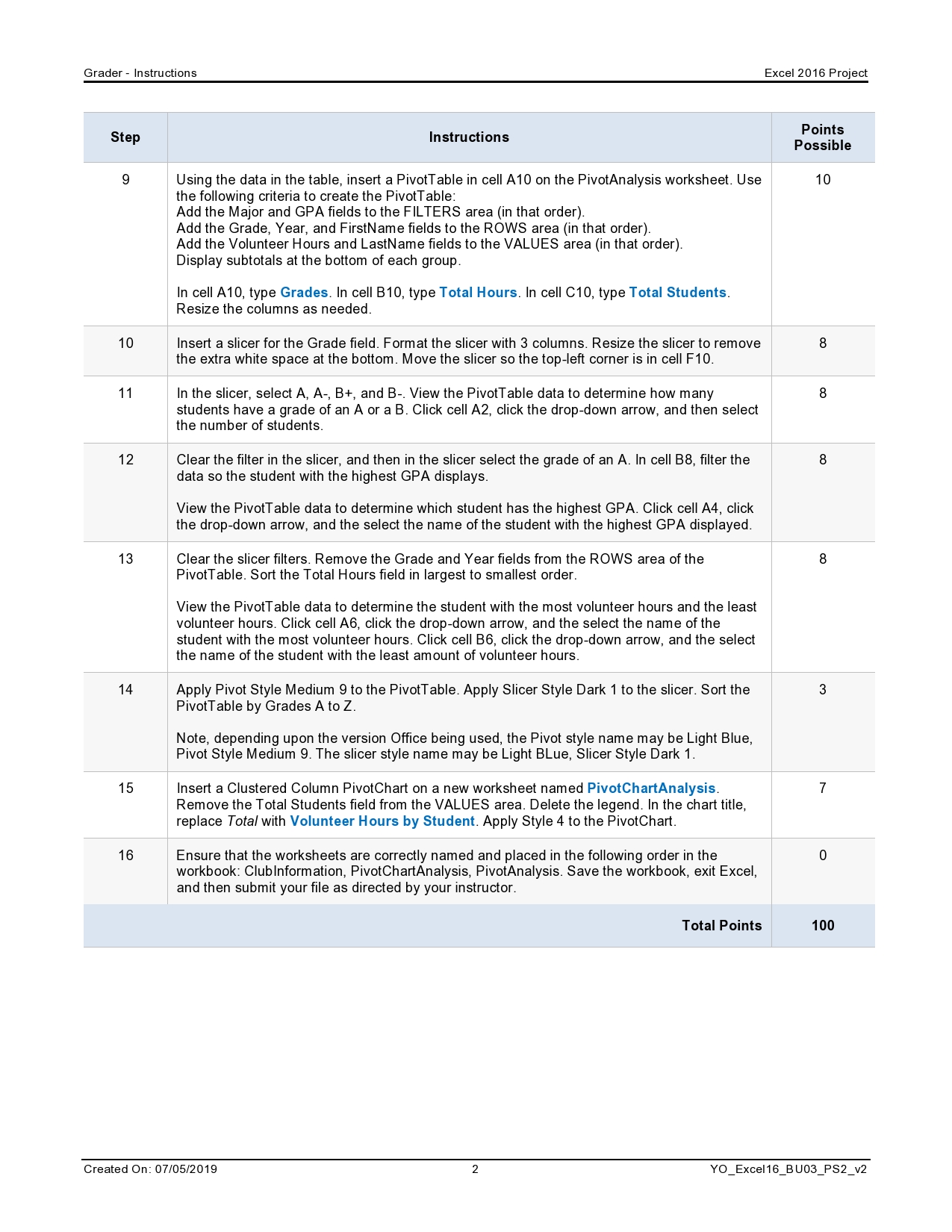
Grader - Instructions Excel 2016 Project Step Instructions Points Possible 9 Using the data in the table, insert a PivotTable in cell A10 on the PivotAnalysis worksheet. Use 10 the following criteria to create the PivotTable: Add the Major and GPA fields to the FILTERS area (in that order). Add the Grade, Year, and FirstName fields to the ROWS area (in that order). Add the Volunteer Hours and LastName fields to the VALUES area (in that order). Display subtotals at the bottom of each group In cell A10, type Grades. In cell B10, type Total Hours. In cell C10, type Total Students Resize the columns as needed. 10 Insert a slicer for the Grade field. Format the slicer with 3 columns. Resize the slicer to remove OO the extra white space at the bottom. Move the slicer so the top-left corner is in cell F10 11 In the slicer, select A, A-, B+, and B-. View the PivotTable data to determine how many students have a grade of an A or a B. Click cell A2, click the drop-down arrow, and then select the number of students 12 Clear the filter in the slicer, and then in the slicer select the grade of an A. In cell B8, filter the 8 data so the student with the highest GPA displays. View the PivotTable data to determine which student has the highest GPA. Click cell A4, click the drop-down arrow, and the select the name of the student with the highest GPA displayed. 13 Clear the slicer filters. Remove the Grade and Year fields from the ROWS area of the 00 PivotTable. Sort the Total Hours field in largest to smallest order. View the PivotTable data to determine the student with the most volunteer hours and the least volunteer hours. Click cell A6, click the drop-down arrow, and the select the name of the student with the most volunteer hours. Click cell B6, click the drop-down arrow, and the select the name of the student with the least amount of volunteer hours 14 Apply Pivot Style Medium 9 to the PivotTable. Apply Slicer Style Dark 1 to the slicer. Sort the 3 PivotTable by Grades A to Z. Note, depending upon the version Office being used, the Pivot style name may be Light Blue, Pivot Style Medium 9. The slicer style name may be Light Blue, Slicer Style Dark 1. 15 Insert a Clustered Column PivotChart on a new worksheet named PivotChartAnalysis. 7 Remove the Total Students field from the VALUES area. Delete the legend. In the chart title, replace Total with Volunteer Hours by Student. Apply Style 4 to the PivotChart. 16 Ensure that the worksheets are correctly named and placed in the following order in the workbook: ClubInformation, PivotChartAnalysis, PivotAnalysis. Save the workbook, exit Excel, O and then submit your file as directed by your instructor. Total Points 100 Created On: 07/05/2019 2 YO_Excel16_BU03_PS2_v2