Greedy Residual Fitting question:
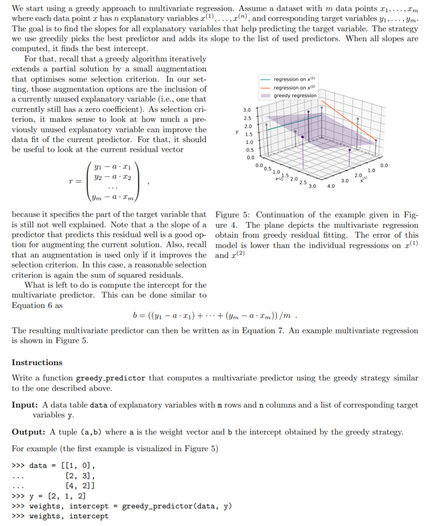
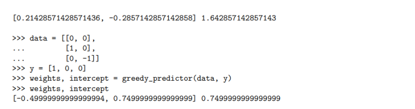
We start using a greedy approach to multivariate regression. Assume a dataset with m data points 1, ..., I'm where each data point r has n explanatory variables r(),..., r("), and corresponding target variables y1, . .. , ym. The goal is to find the slopes for all explanatory variables that help predicting the target variable. The strategy we use greedily picks the best predictor and adds its slope to the list of used predictors. When all slopes are computed, it finds the best intercept. For that, recall that a greedy algorithm iteratively extends a partial solution by a small augmentation that optimises some selection criterion. In our set- regression on x(1) ting, those augmentation options are the inclusion of regression on x(21 a currently unused explanatory variable (i.e., one that greedy regression currently still has a zero coefficient). As selection cri- 3.0 terion, it makes sense to look at how much a pre- 2.5 viously unused explanatory variable can improve the 2.0 data fit of the current predictor. For that, it should 1.5 1.0 be useful to look at the current residual vector 0.5 0.0 y1 - a . T1 1.0 0.0 r = y2 - a . 12 0.0 0.5 1.0 1.5 2.0 2.5 3.0 4.0 3.0 2.0 a . I'm because it specifies the part of the target variable that Figure 5: Continuation of the example given in Fig- is still not well explained. Note that a the slope of a ure 4. The plane depicts the multivariate regression predictor that predicts this residual well is a good op- obtain from greedy residual fitting. The error of this tion for augmenting the current solution. Also, recall model is lower than the individual regressions on r(1) that an augmentation is used only if it improves the and r(2) selection criterion. In this case, a reasonable selection criterion is again the sum of squared residuals. What is left to do is compute the intercept for the multivariate predictor. This can be done similar to Equation 6 as b = ((31 - a . x1) + ...+ (Um -a . I'm)) /m . The resulting multivariate predictor can then be written as in Equation 7. An example multivariate regression is shown in Figure 5. Instructions Write a function greedy predictor that computes a multivariate predictor using the greedy strategy similar to the one described above. Input: A data table data of explanatory variables with m rows and n columns and a list of corresponding target variables y. Output: A tuple (a, b) where a is the weight vector and b the intercept obtained by the greedy strategy. For example (the first example is visualized in Figure 5) >> > data = [[1, 0] , . . [2, 3], . . [4, 2]] >>> y = [2, 1, 2] >>> weights, intercept = greedy_predictor(data, y) >>> weights, intercept\f