h$.$ Apply the Accounting Number Format with $0$ digits after the decimal

to cells B$4$:E$6.$

i$.$ Autofit columns A:E$.$

Calculate total sales for each of the truck locations.

a$.$ Enter the word Total in cell A$7.$

b$.$ Enter a SUM function in cell B$7$ to calculate the total of cells B$4$:B$6.$

c$.$ Use AutoFill to copy the formula to cells C$7$:E$7.$

d$.$ Apply the Total cell style to cells A$7$:E$7.$

$$ Insert a pie chart $(2-$D Pie$)$ to show the Old Bay sales for the month by

location. Each piece of the pie should represent the Old Bay sales for a

single location.

Note: You must complete this step correctly in order to receive points for

completing the next step. Check your work carefully.

Modify the pie chart as follows:

a$.$ Apply the Layout $6$ Quick Layout.

b$.$ Move the chart so it appears below the sales data.

$$ Insert a clustered column chart $(2-$D Column$)$ to show the sales for each

type of popcorn for each location. Do not include the totals.

Note: You must complete this step correctly in order to receive points for

completing the next step. Check your work carefully.

Modify the column chart as follows:

a$.$ If necessary, modify the chart so each location is represented by a data

series and the popcorn types are listed along the $x$ axis.

b$.$ Change the chart title to: July Sales by Popcorn Type

c$.$ Apply the Style $5$ chart Quick Style.

d$.$ Display the chart data labels using the Outside End option.

e$.$ If necessary, move the chart so it is next to the pie chart and the top of

the charts are aligned.

Preview how the worksheet will look when printed, and then apply print

settings to print the worksheet on a single page. Hint: If you have one of the

charts selected, deselect it before previewing the worksheet. Preview the

worksheet again when you are finished to check your work.

a$.$ Change the orientation so the page is wider than it is tall.

b$.$ Change the margins to the preset narrow option.

c$.$ Change the printing scale so all columns will print on a single page.

Top't Corn is considering a new truck purchase. Calculate the monthly loan

payments and total costof the loan.

a$.$ Insert a new worksheet between the MobileSales sheet and the

Onlinesales sheets.

b$.$ OName the new worksheet: TruckLoan

c$.$ Change the color of the worksheet tab to Orange. Use the third color

from the left in the row of Standard colors.

d$.$ Enter the loan terms as shown below.

e$.$ AutoFit column A$.$

f$.$ Set the width of column B to $16.$

g$.$ Apply the Currency number format to cell B$1.$ Display two digits after the

decimal.

h$.$ Enter a formula using the PMT function in cell B$4.$ Be sure to use a

negative value for the

$Pv$ argument.

i$.$ In cell A$6,$ type: Total payments

j$.$ In cell B$6,$ enter a formula to calculate the total paid over the life of the

loan $($the monthly payment amount $*$ the number of payments$).$ Use cell

references.

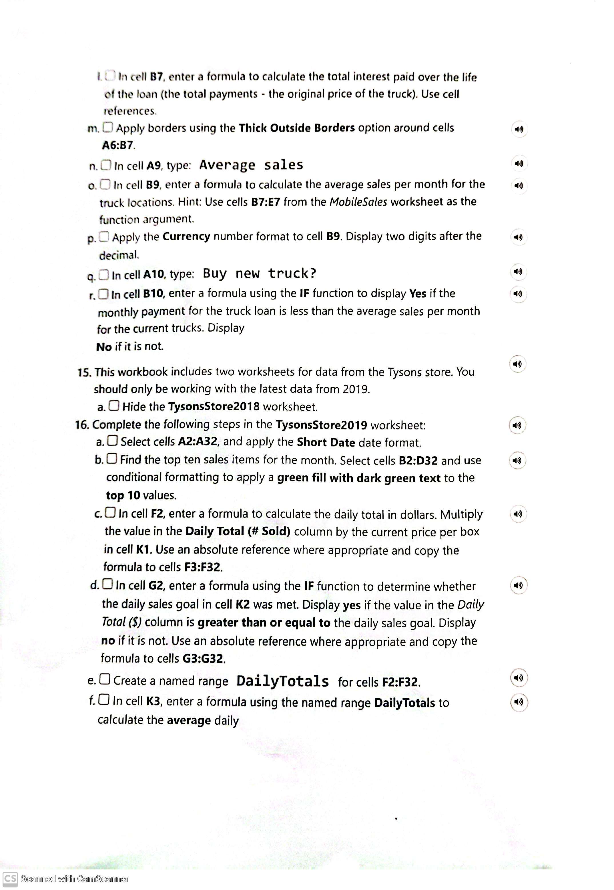
k$.$ In cell A$7,$ type: Interest paid$1\mathrm{.}1$ In cell B$7,$ enter a formula to calculate the total interest paid over the life

of the loan $($the total payments $-$ the original price of the truck$).$ Use cell

references.

m$.$ Apply borders using the Thick Outside Borders option around cells

A$6$:B$7.$

n$.$ In cell A$9,$ type: Average sales

o$.$ In cell B$9,$ enter a formula to calculate the average sales per month for the

truck locations. Hint: Use cells B$7$:E$7$ from the MobileSales worksheet as the

function argument.

p$.$ Apply the Currency number format to cell B$9.$ Display two digits after the

decimal.

q$.$ In cell A$10,$ type: Buy new truck?

r$.$ In cell B$10,$ enter a formula using the IF function to display Yes if the

monthly payment for the truck loan is less than the average sales per month

for the current trucks. Display

No if it is not.

This workbook includes two worksheets for data from the Tysons store. You

should only be working with the latest data from $2019.$

a$.$ Hide the TysonsStore$2018$ worksheet.

Complete the following steps in the TysonsStore$2019$ worksheet:

a$.$ Select cells A$2$:A$32,$ and apply the Short Date date format.

b$.$ Find the top te