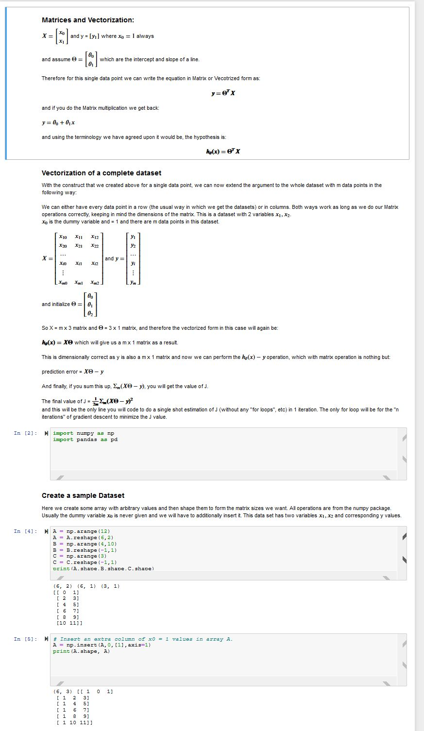
Having trouble with this homework, will give positive review.

Thanks!

file:///C:/Users/SAMBRY~1/AppData/Local/Temp/INFO_4150_Lin_Reg_Teach.html

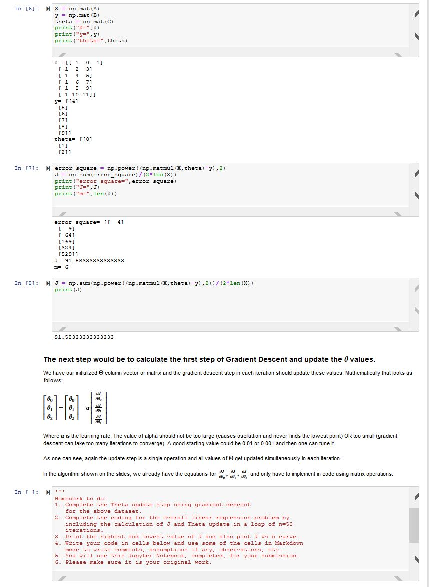
Matrices and Vectorization: y = [y] where Xo = 1 always and assume = which are the intercept and slope of a line. Therefore for this single data point we can write the equation in Matrix or Vecotrized form as: yrex and if you do the Matrix multiplication we get back: y = 0, +0,3 and using the terminology we have agreed upon it would be, the hypothesis is: ho(x)= x Vectorization of a complete dataset With the construct that we created above for a single data point, we can now extend the argument to the whole dataset with m data points in the following way: We can either have every data point in a row (the usual way in which we get the datasets) or in columns. Both ways work as long as we do our Matrix operations correctly, keeping in mind the dimensions of the matrix. This is a dataset with 2 variables X1, X2. Xo is the dummy variable and = 1 and there are m data points in this dataset. X10 X11X12 and y= and initialize = and intialize 8 = So X = mx 3 matrix and = 3 x 1 matrix, and therefore the vectorized form in this case will again be: ho(x) = xe which will give us a mx 1 matrix as a result This is dimensionally correct as y is also a mx 1 matrix and now we can perform the ho(x) - y operation, which with matrix operation is nothing but: prediction error = Xe- y And finally, if you sum this up, Em(XO-y), you will get the value of J. The final value of J = x (xe- y)2 and this will be the only line you will code to do a single shot estimation of J (without any "for loops", etc) in 1 iteration. The only for loop will be for the "n iterations of gradient descent to minimize the J value. In [2]: Nimport numpy as np import pandas as pd Create a sample Dataset Here we create some array with arbitrary values and then shape them to form the matrix sizes we want. All operations are from the numpy package. Usually the dummy variable xo is never given and we will have to additionally insert it. This data set has two variables x1, x2 and corresponding y values. In [4]: NA = np.arange (12) A = A. reshape (6,2) B = np.arange (4,10) B = B.reshape(-1,1) C = np.arange (3) C = C.reshape (-1,1) print (A.shape. B. shape. C.shape) (3, 1) 16, 2) (6, 1) [[ 0 1] [ 2 3] (4 51 [6 71 [89] [10 111] In [5]: N# Insert an extra column of x0 = 1 values in array A. A = np.insert (A, 0, [1], axis=1) print (A.shape, A) 0 1] (6, 3) [[ 1 [ 1 2 3] [145] ( 1 6 7] [189] [ 1 10 11]1 In [6]: NX = np. mat (A) y = p.That () theta = np. mat (C) print ("X=",X) print("y=", y) print("theta=", theta) X= [[ 1 0 1] [ 1 2 31 [145] [ 1 6 7] [189] [ 1 10 11]] y= [[4] (5) 161 [7] [8] [91 theta= [[0] [1] [2]1 In [7]: N error_square = np.power( (np.matmul(x, theta)-y), 2) J = np.gum error_square)/(2*len(X)) print("error square=", error_square) print("J=",J) print("m=", len(X)) error square= [ 4] [ 9] [64] [169] [324] [52911 J= 91.58333333333333 m= 6 In [@]: N J = np. sum (np. power ( (np.matmul (X, theta)-y), 2))/(2*len (X)) print (J) 91.58333333333333 The next step would be to calculate the first step of Gradient Descent and update the values. column vector or matrix and the gradient descent step in each iteration should update these values. Mathematically that looks as We have our initialized follows: [ 0 ] [ 0 ] 0, = 02 021 Where a is the learning rate. The value of alpha should not be too large (causes oscilattion and never finds the lowest point) OR too small (gradient descent can take too many iterations to converge). A good starting value could be 0.01 or 0.001 and then one can tune it. As one can see, again the update step is a single operation and all values of get updated simultaneously in each iteration. In the algorithm shown on the slides, we already have the equations for and only have to implement in code using matrix operations. In [ ]: N Homework to do: 1. Complete the Theta update step using gradient descent for the above dataset. 2. Complete the coding for the overall linear regression problem by including the calculation of J and Theta update in a loop of n=50 iterations. 3. Print the highest and lowest value of J and also plotu vs n curve 4. Write your code in cells below and use some of the cells in Markdown mode to write comments, assumptions if any, observations, etc. 5. You will use this Jupyter Notebook, completed, for your submission. 6. Please make sure it is your original work. Matrices and Vectorization: y = [y] where Xo = 1 always and assume = which are the intercept and slope of a line. Therefore for this single data point we can write the equation in Matrix or Vecotrized form as: yrex and if you do the Matrix multiplication we get back: y = 0, +0,3 and using the terminology we have agreed upon it would be, the hypothesis is: ho(x)= x Vectorization of a complete dataset With the construct that we created above for a single data point, we can now extend the argument to the whole dataset with m data points in the following way: We can either have every data point in a row (the usual way in which we get the datasets) or in columns. Both ways work as long as we do our Matrix operations correctly, keeping in mind the dimensions of the matrix. This is a dataset with 2 variables X1, X2. Xo is the dummy variable and = 1 and there are m data points in this dataset. X10 X11X12 and y= and initialize = and intialize 8 = So X = mx 3 matrix and = 3 x 1 matrix, and therefore the vectorized form in this case will again be: ho(x) = xe which will give us a mx 1 matrix as a result This is dimensionally correct as y is also a mx 1 matrix and now we can perform the ho(x) - y operation, which with matrix operation is nothing but: prediction error = Xe- y And finally, if you sum this up, Em(XO-y), you will get the value of J. The final value of J = x (xe- y)2 and this will be the only line you will code to do a single shot estimation of J (without any "for loops", etc) in 1 iteration. The only for loop will be for the "n iterations of gradient descent to minimize the J value. In [2]: Nimport numpy as np import pandas as pd Create a sample Dataset Here we create some array with arbitrary values and then shape them to form the matrix sizes we want. All operations are from the numpy package. Usually the dummy variable xo is never given and we will have to additionally insert it. This data set has two variables x1, x2 and corresponding y values. In [4]: NA = np.arange (12) A = A. reshape (6,2) B = np.arange (4,10) B = B.reshape(-1,1) C = np.arange (3) C = C.reshape (-1,1) print (A.shape. B. shape. C.shape) (3, 1) 16, 2) (6, 1) [[ 0 1] [ 2 3] (4 51 [6 71 [89] [10 111] In [5]: N# Insert an extra column of x0 = 1 values in array A. A = np.insert (A, 0, [1], axis=1) print (A.shape, A) 0 1] (6, 3) [[ 1 [ 1 2 3] [145] ( 1 6 7] [189] [ 1 10 11]1 In [6]: NX = np. mat (A) y = p.That () theta = np. mat (C) print ("X=",X) print("y=", y) print("theta=", theta) X= [[ 1 0 1] [ 1 2 31 [145] [ 1 6 7] [189] [ 1 10 11]] y= [[4] (5) 161 [7] [8] [91 theta= [[0] [1] [2]1 In [7]: N error_square = np.power( (np.matmul(x, theta)-y), 2) J = np.gum error_square)/(2*len(X)) print("error square=", error_square) print("J=",J) print("m=", len(X)) error square= [ 4] [ 9] [64] [169] [324] [52911 J= 91.58333333333333 m= 6 In [@]: N J = np. sum (np. power ( (np.matmul (X, theta)-y), 2))/(2*len (X)) print (J) 91.58333333333333 The next step would be to calculate the first step of Gradient Descent and update the values. column vector or matrix and the gradient descent step in each iteration should update these values. Mathematically that looks as We have our initialized follows: [ 0 ] [ 0 ] 0, = 02 021 Where a is the learning rate. The value of alpha should not be too large (causes oscilattion and never finds the lowest point) OR too small (gradient descent can take too many iterations to converge). A good starting value could be 0.01 or 0.001 and then one can tune it. As one can see, again the update step is a single operation and all values of get updated simultaneously in each iteration. In the algorithm shown on the slides, we already have the equations for and only have to implement in code using matrix operations. In [ ]: N Homework to do: 1. Complete the Theta update step using gradient descent for the above dataset. 2. Complete the coding for the overall linear regression problem by including the calculation of J and Theta update in a loop of n=50 iterations. 3. Print the highest and lowest value of J and also plotu vs n curve 4. Write your code in cells below and use some of the cells in Markdown mode to write comments, assumptions if any, observations, etc. 5. You will use this Jupyter Notebook, completed, for your submission. 6. Please make sure it is your original work