Question
he following is the built-in humps function that MATLAB uses to demonstrate some of its numerical capabilities: f ( x )= 1 + 1 6
he following is the built-in humps function that MATLAB uses to demonstrate some of its numerical capabilities:
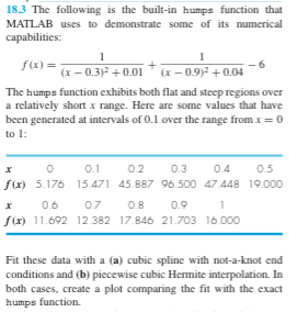
f(x)= 1 + 1 6 (x 0.3)2 +0.01 (x 0.9)2 +0.04
The humps function exhibits both flat and steep regions over a relatively short x range. Here are some values that have been generated at intervals of 0.1 over the range from x = 0 to 1:
x00.10.20.30.40.5
f(x) 5.176 15.471 45.887 96.500 47.448 19.000
x 0.6 0.7 0.8 0.9 1 f (x) 11.692 12.382 17.846 21.703 16.000
Fit these data with a (a) cubic spline with not-a-knot end conditions and (b) piecewise cubic Hermite interpolation. In both cases, create a plot comparing the fit with the exact humps function.

Step by Step Solution
There are 3 Steps involved in it
Step: 1

Get Instant Access to Expert-Tailored Solutions
See step-by-step solutions with expert insights and AI powered tools for academic success
Step: 2

Step: 3

Ace Your Homework with AI
Get the answers you need in no time with our AI-driven, step-by-step assistance
Get Started


