Hello, Hope you are doing well. So we were given this MOCK assessment to help us prepare for our upcoming midterm. I have been struggling with the concepts and problems and was wondering if someone would be able to solve this problem, but also provide step by step solution so that I can follow how you solved the problem?
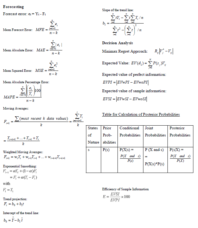
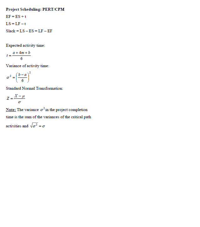
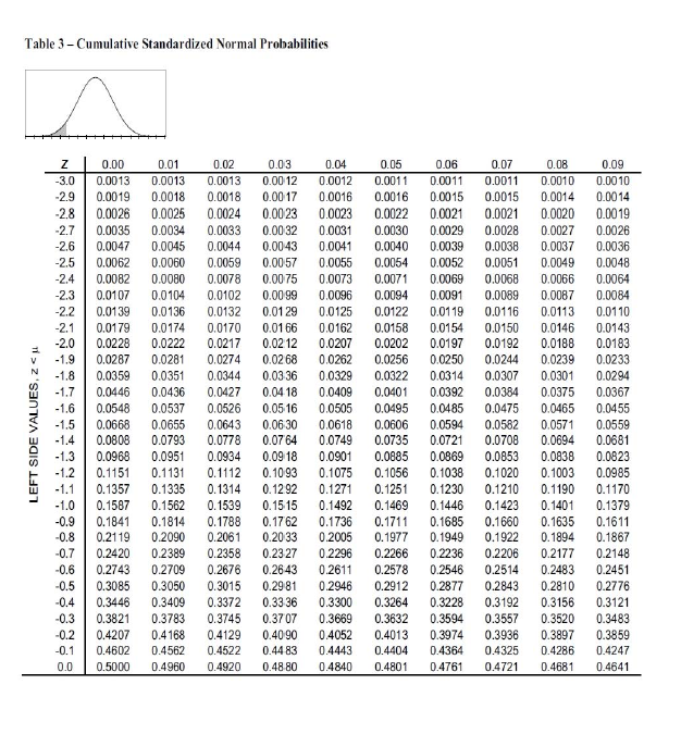
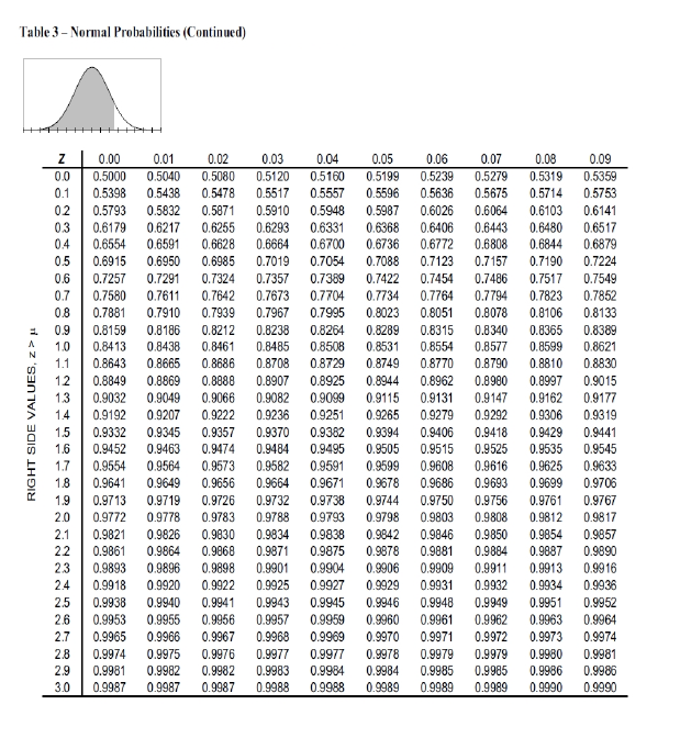
I have attached files with formulas that we may use to potentially solving the problem and distribution tables given the question.


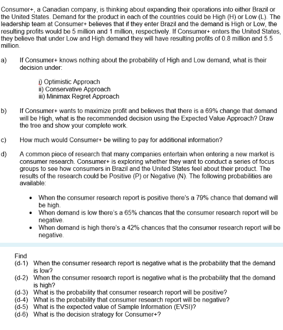
Consumer-, a Canadian company, is thinking about expanding their operations into either Brazil or the United States. Demand for the product in each of the countries could be High (H) or Low (L). The leadership team at Consumer+ believes that if they enter Brazil and the demand is High or Low, the resulting profits would be 5 million and 1 million, respectively. If Consumer+ enters the United States, they believe that under Low and High demand they will have resulting profits of 0.8 million and 5.5 million a) If Consumer+ knows nothing about the probability of High and Low demand, what is their decision under: D Optimistic Approach ii) Conservative Approach ii) Minimax Regret Approach b) If Consumer+ wants to maximize profit and believes that there is a 69% change that demand will be High, what is the recommended decision using the Expected Value Approach? Draw the tree and show your complete work. c) How much would Consumer+ be willing to pay for additional information? d) A common piece of research that many companies entertain when entering a new market is consumer research. Consumer+ is exploring whether they want to conduct a series of focus groups to see how consumers in Brazil and the United States feel about their product. The results of the research could be Positive (P) or Negative (N). The following probabilities are available When the consumer research report is positive there's a 79% chance that demand will be high When demand is low there's a 65% chances that the consumer research report will be negative When demand is high there's a 42% chances that the consumer research report will be negative Find (d-1) When the consumer research report is negative what is the probability that the demand is low? (4-2) When the consumer research report is negative what is the probability that the demand is high? (0-3) What is the probability that consumer research report will be positive? (0-4) What is the probability that consumer research report will be negative? (d-5) What is the expected value of Sample Information (EVSI)? (d-6) What is the decision strategy for Consumer+? Forecasting Forecast error: et = Yt - Ft Slope of the trend line: ty, - ZY,In -! b = fak! Mean Forecast Error: MFE =- n-k Sle, Mean Absolute Error: MAE = n-k Sep Mean Squared Error: MSE ==+1 n-k Decision Analysis Minimax Regret Approach: R|1-V,| Expected Value: EV(d,)$P(,), Expected value of perfect information: EVPI =|EVWPI EYWOPI Expected value of sample information: EVSI = |EVWSI EVwo.SI Mean Absolute Percentage Error: R 09.00 MAPE n- Moving Averages: (most recent k data values) Table for Calculation of Posterior Probabilities F- k Conditional Joint Posterior Probabilities Probabilities Probabilities Y;-*+2+...+Y4 +Y, States Prior of Prob- Nature abilities P(s) k S Weighted Moving Averages: F. - = w,Y, +w-Y2+...+W-*-*-*=1 P(X) = PCX and 3) P(3) PX and s) P(X) = PCX and 3) P() P(X|s)*P(5) Exponential Smoothing: F+1 = al. +(1-a) = F; + a(Y,-F) with F = Y Efficiency of Sample Information EVSI EVPI x 100 Trend projection: F = b + b1 Intercept of the trend line: bo = Y-bi Project Scheduling: PERT/CPM EF = ES +t LS = LF-t Slack = LS-ES-LF - EF Expected activity time: a + 4m + b 6 Variance of activity time: = b-a o-on Standard Normal Transformation: X- Z Note: The variance oin the project completion time is the sum of the variances of the critical path activities and Vo?=0 Table 3 - Cumulative Standardized Normal Probabilities LEFT SIDE VALUES, Zu Z -3.0 -2.9 -2.8 -2.7 -2.6 -2.5 -2.4 -2.3 -2.2 -2.1 -2.0 -1.9 -1.8 -1.7 -1.6 -1.5 -1.4 -1.3 - 1.2 -1.1 - 1.0 -0.9 -0.8 -0.7 -0.6 -0.5 -0.4 -0.3 -0.2 -0.1 0.0 0.00 0.0013 0.0019 0.0026 0.0035 0.0047 0.0062 0.0082 0.0107 0.0139 0.0179 0.0228 0.0287 0.0359 0.0446 0.0548 0.0668 0.0808 0.0968 0.1151 0.1357 0.1587 0.1841 0.2119 0.2420 0.2743 0.3085 0.3446 0.3821 0.4207 0.4602 0.5000 0.01 0.0013 0.0018 0.0025 0.0034 0.0045 0.0060 0.0080 0.0104 0.0136 0.0174 0.0222 0.0281 0.0351 0.0436 0.0537 0.0655 0.0793 0.0951 0.1131 0.1335 0.1562 0.1814 0.2090 0.2389 0.2709 0.3050 0.3409 0.3783 0.4168 0.4562 0.4960 0.02 0.0013 0.0018 0.0024 0.0033 0.0044 0.0059 0.0078 0.0102 0.0132 0.0170 0.0217 0.0274 0.0344 0.0427 0.0526 0.0643 0.0778 0.0934 0.1112 0.1314 0.1539 0.1788 0.2061 0.2358 0.2676 0.3015 0.3372 0.3745 0.4129 0.4522 0.4920 0.03 0.00 12 0.0017 0.0023 0.0032 0.0043 0.0057 0.00 75 0.00 99 0.0129 0.0166 0.02 12 0.0268 0.03 36 0.0418 0.0516 0.0630 0.07 64 0.0918 0.1093 0.12 92 0.1515 0.1762 0.2033 0.23 27 0.26 43 0.2981 0.3336 0.3707 0.40 90 0.4483 0.48 80 0.04 0.0012 0.0016 0.0023 0.0031 0.0041 0.0055 0.0073 0.0096 0.0125 0.0162 0.0207 0.0262 0.0329 0.0409 0.0505 0.0618 0.0749 0.0901 0.1075 0.1271 0.1492 0.1736 0.2005 0.2296 0.2611 0.2946 0.3300 0.3669 0.4052 0.4443 0.4840 0.05 0.0011 0.0016 0.0022 0.0030 0.0040 0.0054 0.0071 0.0094 0.0122 0.0158 0.0202 0.0256 0.0322 0.0401 0.0495 0.0606 0.0735 0.0885 0.1056 0.1251 0.1469 0.1711 0.1977 0.2266 0.2578 0.2912 0.3264 0.3632 0.4013 0.4404 0.4801 0.06 0.0011 0.0015 0.0021 0.0029 0.0039 0.0052 0.0069 0.0091 0.0119 0.0154 0.0197 0.0250 0.0314 0.0392 0.0485 0.0594 0.0721 0.0869 0.1038 0.1230 0.1446 0.1685 0.1949 0.2236 0.2546 0.2877 0.3228 0.3594 0.3974 0.4364 0.4761 0.07 0.0011 0.0015 0.0021 0.0028 0.0038 0.0051 0.0068 0.0089 0.0116 0.0150 0.0192 0.0244 0.0307 0.0384 0.0475 0.0582 0.0708 0.0853 0.1020 0.1210 0.1423 0.1660 0.1922 0.2206 0.2514 0.2843 0.3192 0.3557 0.3936 0.4325 0.4721 0.08 0.0010 0.0014 0.0020 0.0027 0.0037 0.0049 0.0066 0.0087 0.0113 0.0146 0.0188 0.0239 0.0301 0.0375 0.0465 0.0571 0.0694 0.0838 0.1003 0.1190 0.1401 0.1635 0.1894 0.2177 0.2483 0.2810 0.3156 0.3520 0.3897 0.4286 0.4681 0.09 0.0010 0.0014 0.0019 0.0026 0.0036 0.0048 0.0064 0.0084 0.0110 0.0143 0.0183 0.0233 0.0294 0.0367 0.0455 0.0559 0.0681 0.0823 0.0985 0.1170 0.1379 0.1611 0.1867 0.2148 0.2451 0.2776 0.3121 0.3483 0.3859 0.4247 0.4641 Table 3 - Normal Probabilities (Continued) RIGHT SIDE VALUES, Z> Z 0.0 0.1 02 03 0.4 0.5 0.6 0.7 0.8 0.9 1.0 1.1 12 13 1.4 1.5 1.6 1.7 1.8 1.9 2.0 2.1 22 23 2.4 25 26 2.7 2.8 2.9 3.0 0.00 0.5000 0.5398 0.5793 0.6179 0.6554 0.6915 0.7257 0.7580 0.7881 0.8159 0.8413 0.8643 0.8849 0.9032 0.9192 0.9332 0.9452 0.9554 0.9641 0.9713 0.9772 0.9821 0.9861 0.9893 0.9918 0.9938 0.9953 0.9965 0.9974 0.9981 0.9987 0.01 0.5040 0.5438 0.5832 0.6217 0.6591 0.6950 0.7291 0.7611 0.7910 0.8186 0.8438 0.8665 0.8869 0.9049 0.9207 0.9345 0.9463 0.9564 0.9649 0.9719 0.9778 0.9826 0.9864 0.9896 0.9920 0.9940 0.9955 0.9966 0.9975 0.9982 0.9987 0.02 0.5080 0.5478 0.5871 0.6255 0.6628 0.6985 0.7324 0.7642 0.7939 0.8212 0.8461 0.8686 0.8888 0.9066 0.9222 0.9357 0.9474 0.9573 0.9656 0.9726 0.9783 0.9830 0.9868 0.9898 0.9922 0.9941 0.9956 0.9967 0.9976 0.9982 0.9987 0.03 0.5120 0.5517 0.5910 0.6293 0.6664 0.7019 0.7357 0.7673 0.7967 0.8238 0.8485 0.8708 0.8907 0.9082 0.9236 0.9370 0.9484 0.9582 0.9664 0.9732 0.9788 0.9834 0.9871 0.9901 0.9925 0.9943 0.9957 0.9968 0.9977 0.9983 0.9988 0.04 0.5160 0.5557 0.5948 0.6331 0.6700 0.7054 0.7389 0.7704 0.7995 0.8264 0.8508 0.8729 0.8925 0.9099 0.9251 0.9382 0.9495 0.9591 0.9671 0.9738 0.9793 0.9838 0.9875 0.9904 0.9927 0.9945 0.9959 0.9969 0.9977 0.9984 0.9988 0.05 0.5199 0.5596 0.5987 0.6368 0.6736 0.7088 0.7422 0.7734 0.8023 0.8289 0.8531 0.8749 0.8944 0.9115 0.9265 0.9394 0.9505 0.9599 0.9678 0.9744 0.9798 0.9842 0.9878 0.9906 0.9929 0.9946 0.9960 0.9970 0.9978 0.9984 0.9989 0.06 0.5239 0.5636 0.6026 0.6406 0.6772 0.7123 0.7454 0.7764 0.8051 0.8315 0.8554 0.8770 0.8962 0.9131 0.9279 0.9406 0.9515 0.9608 0.9686 0.9750 0.9803 0.9846 0.9881 0.9909 0.9931 0.9948 0.9961 0.9971 0.9979 0.9985 0.9989 0.07 0.5279 0.5675 0.6064 0.6443 0.6808 0.7157 0.7486 0.7794 0.8078 0.8340 0.8577 0.8790 0.8980 0.9147 0.9292 0.9418 0.9525 0.9616 0.9693 0.9756 0.9808 0.9850 0.9884 0.9911 0.9932 0.9949 0.9962 0.9972 0.9979 0.9985 0.9989 0.08 0.5319 0.5714 0.6103 0.6480 0.6844 0.7190 0.7517 0.7823 0.8106 0.8365 0.8599 0.8810 0.8997 0.9162 0.9306 0.9429 0.9535 0.9625 0.9699 0.9761 0.9812 0.9854 0.9887 0.9913 0.9934 0.9951 0.9963 0.9973 0.9980 0.9986 0.9990 0.09 0.5359 0.5753 0.6141 0.6517 0.6879 0.7224 0.7549 0.7852 0.8133 0.8389 0.8621 0.8830 0.9015 0.9177 0.9319 0.9441 0.9545 0.9633 0.9706 0.9767 0.9817 0.9857 0.9890 0.9916 0.9938 0.9952 0.9964 0.9974 0.9981 0.9986 0.9990 Consumer-, a Canadian company, is thinking about expanding their operations into either Brazil or the United States. Demand for the product in each of the countries could be High (H) or Low (L). The leadership team at Consumer+ believes that if they enter Brazil and the demand is High or Low, the resulting profits would be 5 million and 1 million, respectively. If Consumer+ enters the United States, they believe that under Low and High demand they will have resulting profits of 0.8 million and 5.5 million a) If Consumer+ knows nothing about the probability of High and Low demand, what is their decision under: D Optimistic Approach ii) Conservative Approach ii) Minimax Regret Approach b) If Consumer+ wants to maximize profit and believes that there is a 69% change that demand will be High, what is the recommended decision using the Expected Value Approach? Draw the tree and show your complete work. c) How much would Consumer+ be willing to pay for additional information? d) A common piece of research that many companies entertain when entering a new market is consumer research. Consumer+ is exploring whether they want to conduct a series of focus groups to see how consumers in Brazil and the United States feel about their product. The results of the research could be Positive (P) or Negative (N). The following probabilities are available When the consumer research report is positive there's a 79% chance that demand will be high When demand is low there's a 65% chances that the consumer research report will be negative When demand is high there's a 42% chances that the consumer research report will be negative Find (d-1) When the consumer research report is negative what is the probability that the demand is low? (4-2) When the consumer research report is negative what is the probability that the demand is high? (0-3) What is the probability that consumer research report will be positive? (0-4) What is the probability that consumer research report will be negative? (d-5) What is the expected value of Sample Information (EVSI)? (d-6) What is the decision strategy for Consumer+? Forecasting Forecast error: et = Yt - Ft Slope of the trend line: ty, - ZY,In -! b = fak! Mean Forecast Error: MFE =- n-k Sle, Mean Absolute Error: MAE = n-k Sep Mean Squared Error: MSE ==+1 n-k Decision Analysis Minimax Regret Approach: R|1-V,| Expected Value: EV(d,)$P(,), Expected value of perfect information: EVPI =|EVWPI EYWOPI Expected value of sample information: EVSI = |EVWSI EVwo.SI Mean Absolute Percentage Error: R 09.00 MAPE n- Moving Averages: (most recent k data values) Table for Calculation of Posterior Probabilities F- k Conditional Joint Posterior Probabilities Probabilities Probabilities Y;-*+2+...+Y4 +Y, States Prior of Prob- Nature abilities P(s) k S Weighted Moving Averages: F. - = w,Y, +w-Y2+...+W-*-*-*=1 P(X) = PCX and 3) P(3) PX and s) P(X) = PCX and 3) P() P(X|s)*P(5) Exponential Smoothing: F+1 = al. +(1-a) = F; + a(Y,-F) with F = Y Efficiency of Sample Information EVSI EVPI x 100 Trend projection: F = b + b1 Intercept of the trend line: bo = Y-bi Project Scheduling: PERT/CPM EF = ES +t LS = LF-t Slack = LS-ES-LF - EF Expected activity time: a + 4m + b 6 Variance of activity time: = b-a o-on Standard Normal Transformation: X- Z Note: The variance oin the project completion time is the sum of the variances of the critical path activities and Vo?=0 Table 3 - Cumulative Standardized Normal Probabilities LEFT SIDE VALUES, Zu Z -3.0 -2.9 -2.8 -2.7 -2.6 -2.5 -2.4 -2.3 -2.2 -2.1 -2.0 -1.9 -1.8 -1.7 -1.6 -1.5 -1.4 -1.3 - 1.2 -1.1 - 1.0 -0.9 -0.8 -0.7 -0.6 -0.5 -0.4 -0.3 -0.2 -0.1 0.0 0.00 0.0013 0.0019 0.0026 0.0035 0.0047 0.0062 0.0082 0.0107 0.0139 0.0179 0.0228 0.0287 0.0359 0.0446 0.0548 0.0668 0.0808 0.0968 0.1151 0.1357 0.1587 0.1841 0.2119 0.2420 0.2743 0.3085 0.3446 0.3821 0.4207 0.4602 0.5000 0.01 0.0013 0.0018 0.0025 0.0034 0.0045 0.0060 0.0080 0.0104 0.0136 0.0174 0.0222 0.0281 0.0351 0.0436 0.0537 0.0655 0.0793 0.0951 0.1131 0.1335 0.1562 0.1814 0.2090 0.2389 0.2709 0.3050 0.3409 0.3783 0.4168 0.4562 0.4960 0.02 0.0013 0.0018 0.0024 0.0033 0.0044 0.0059 0.0078 0.0102 0.0132 0.0170 0.0217 0.0274 0.0344 0.0427 0.0526 0.0643 0.0778 0.0934 0.1112 0.1314 0.1539 0.1788 0.2061 0.2358 0.2676 0.3015 0.3372 0.3745 0.4129 0.4522 0.4920 0.03 0.00 12 0.0017 0.0023 0.0032 0.0043 0.0057 0.00 75 0.00 99 0.0129 0.0166 0.02 12 0.0268 0.03 36 0.0418 0.0516 0.0630 0.07 64 0.0918 0.1093 0.12 92 0.1515 0.1762 0.2033 0.23 27 0.26 43 0.2981 0.3336 0.3707 0.40 90 0.4483 0.48 80 0.04 0.0012 0.0016 0.0023 0.0031 0.0041 0.0055 0.0073 0.0096 0.0125 0.0162 0.0207 0.0262 0.0329 0.0409 0.0505 0.0618 0.0749 0.0901 0.1075 0.1271 0.1492 0.1736 0.2005 0.2296 0.2611 0.2946 0.3300 0.3669 0.4052 0.4443 0.4840 0.05 0.0011 0.0016 0.0022 0.0030 0.0040 0.0054 0.0071 0.0094 0.0122 0.0158 0.0202 0.0256 0.0322 0.0401 0.0495 0.0606 0.0735 0.0885 0.1056 0.1251 0.1469 0.1711 0.1977 0.2266 0.2578 0.2912 0.3264 0.3632 0.4013 0.4404 0.4801 0.06 0.0011 0.0015 0.0021 0.0029 0.0039 0.0052 0.0069 0.0091 0.0119 0.0154 0.0197 0.0250 0.0314 0.0392 0.0485 0.0594 0.0721 0.0869 0.1038 0.1230 0.1446 0.1685 0.1949 0.2236 0.2546 0.2877 0.3228 0.3594 0.3974 0.4364 0.4761 0.07 0.0011 0.0015 0.0021 0.0028 0.0038 0.0051 0.0068 0.0089 0.0116 0.0150 0.0192 0.0244 0.0307 0.0384 0.0475 0.0582 0.0708 0.0853 0.1020 0.1210 0.1423 0.1660 0.1922 0.2206 0.2514 0.2843 0.3192 0.3557 0.3936 0.4325 0.4721 0.08 0.0010 0.0014 0.0020 0.0027 0.0037 0.0049 0.0066 0.0087 0.0113 0.0146 0.0188 0.0239 0.0301 0.0375 0.0465 0.0571 0.0694 0.0838 0.1003 0.1190 0.1401 0.1635 0.1894 0.2177 0.2483 0.2810 0.3156 0.3520 0.3897 0.4286 0.4681 0.09 0.0010 0.0014 0.0019 0.0026 0.0036 0.0048 0.0064 0.0084 0.0110 0.0143 0.0183 0.0233 0.0294 0.0367 0.0455 0.0559 0.0681 0.0823 0.0985 0.1170 0.1379 0.1611 0.1867 0.2148 0.2451 0.2776 0.3121 0.3483 0.3859 0.4247 0.4641 Table 3 - Normal Probabilities (Continued) RIGHT SIDE VALUES, Z> Z 0.0 0.1 02 03 0.4 0.5 0.6 0.7 0.8 0.9 1.0 1.1 12 13 1.4 1.5 1.6 1.7 1.8 1.9 2.0 2.1 22 23 2.4 25 26 2.7 2.8 2.9 3.0 0.00 0.5000 0.5398 0.5793 0.6179 0.6554 0.6915 0.7257 0.7580 0.7881 0.8159 0.8413 0.8643 0.8849 0.9032 0.9192 0.9332 0.9452 0.9554 0.9641 0.9713 0.9772 0.9821 0.9861 0.9893 0.9918 0.9938 0.9953 0.9965 0.9974 0.9981 0.9987 0.01 0.5040 0.5438 0.5832 0.6217 0.6591 0.6950 0.7291 0.7611 0.7910 0.8186 0.8438 0.8665 0.8869 0.9049 0.9207 0.9345 0.9463 0.9564 0.9649 0.9719 0.9778 0.9826 0.9864 0.9896 0.9920 0.9940 0.9955 0.9966 0.9975 0.9982 0.9987 0.02 0.5080 0.5478 0.5871 0.6255 0.6628 0.6985 0.7324 0.7642 0.7939 0.8212 0.8461 0.8686 0.8888 0.9066 0.9222 0.9357 0.9474 0.9573 0.9656 0.9726 0.9783 0.9830 0.9868 0.9898 0.9922 0.9941 0.9956 0.9967 0.9976 0.9982 0.9987 0.03 0.5120 0.5517 0.5910 0.6293 0.6664 0.7019 0.7357 0.7673 0.7967 0.8238 0.8485 0.8708 0.8907 0.9082 0.9236 0.9370 0.9484 0.9582 0.9664 0.9732 0.9788 0.9834 0.9871 0.9901 0.9925 0.9943 0.9957 0.9968 0.9977 0.9983 0.9988 0.04 0.5160 0.5557 0.5948 0.6331 0.6700 0.7054 0.7389 0.7704 0.7995 0.8264 0.8508 0.8729 0.8925 0.9099 0.9251 0.9382 0.9495 0.9591 0.9671 0.9738 0.9793 0.9838 0.9875 0.9904 0.9927 0.9945 0.9959 0.9969 0.9977 0.9984 0.9988 0.05 0.5199 0.5596 0.5987 0.6368 0.6736 0.7088 0.7422 0.7734 0.8023 0.8289 0.8531 0.8749 0.8944 0.9115 0.9265 0.9394 0.9505 0.9599 0.9678 0.9744 0.9798 0.9842 0.9878 0.9906 0.9929 0.9946 0.9960 0.9970 0.9978 0.9984 0.9989 0.06 0.5239 0.5636 0.6026 0.6406 0.6772 0.7123 0.7454 0.7764 0.8051 0.8315 0.8554 0.8770 0.8962 0.9131 0.9279 0.9406 0.9515 0.9608 0.9686 0.9750 0.9803 0.9846 0.9881 0.9909 0.9931 0.9948 0.9961 0.9971 0.9979 0.9985 0.9989 0.07 0.5279 0.5675 0.6064 0.6443 0.6808 0.7157 0.7486 0.7794 0.8078 0.8340 0.8577 0.8790 0.8980 0.9147 0.9292 0.9418 0.9525 0.9616 0.9693 0.9756 0.9808 0.9850 0.9884 0.9911 0.9932 0.9949 0.9962 0.9972 0.9979 0.9985 0.9989 0.08 0.5319 0.5714 0.6103 0.6480 0.6844 0.7190 0.7517 0.7823 0.8106 0.8365 0.8599 0.8810 0.8997 0.9162 0.9306 0.9429 0.9535 0.9625 0.9699 0.9761 0.9812 0.9854 0.9887 0.9913 0.9934 0.9951 0.9963 0.9973 0.9980 0.9986 0.9990 0.09 0.5359 0.5753 0.6141 0.6517 0.6879 0.7224 0.7549 0.7852 0.8133 0.8389 0.8621 0.8830 0.9015 0.9177 0.9319 0.9441 0.9545 0.9633 0.9706 0.9767 0.9817 0.9857 0.9890 0.9916 0.9938 0.9952 0.9964 0.9974 0.9981 0.9986 0.9990
