

Help appreciated:-
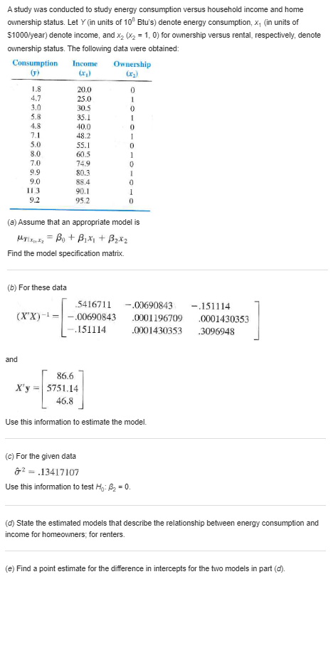
\fConsider the model .11.\" 1.. 1 = {30 + 315'\" + 3212. These data are available: 1': I: JJ 0 E 9 2 '9 E 4 S T {a} Find 3 3 3 3 [2'1 x\" 21 1'2: E Eula E In}; a 7: i=1 a: 3 3 3 3 to) Find the normal equations. to} Show that on = 9, is = _5, and 132 = t] are solutions to the normal equations. In Example 12.2.5, we developed a quadratic regression equation from which the unit cost of producing a drug can be predicted based on the number of units produced. Use the information given there to estimate Var Bo, Var By, and Var B2. Example 12.2.5 These data are available on X, the number of units of drug pro- duced, and I the cost per unit of producing the drug. (See Example 12.1.1.) 5 10 10 15 15 20 20 25 25 14.0 125 7.0 5.0 2.1 1.8 6.2 4.9 13.2 14.6 The model specification matrix for a quadratic model is 5 2.5 25 1 10 100 10 100 15 225 15 225 1 20 400 20 400 25 625 25 625 10 150 2750 X'X 150 2750 $6.250 2750 56.250 1,223,750 81.3 Xy= 1228 24.535 Apart from round-off enor 2.3 -,33 (xx)-= -33 .05342857 -.00171429 01 -,00171429 00005714286 The least-squares estimates for - Bj, By are 27.3 b = (xx) ry= -3.313 -111 The estimated model is Ary - 27.3-3313x + Illx The predicted unit cost of producing 12 units of the drug is 5 = 27.3 - 3.313(12) + .111(12) = 3.528 Example 12.1.1 Suppose that we want to develop an equation with which we can predict the gasoline mileage of an automobile based on its weight and the temperature at the time of operation. We might pose the model Arin. 12 = BotBixt + Batz Here the response variable is Y, the mileage obtained. There are two independent or predictor variables. These are X,, the weight of the car, and X,, the temperature. The values assumed by these variables are denoted by x, and a, respectively. For example, we might want to predict the gas mileage for a car that weighs 1.6 tons when it is be- ing driven in 85" F weather. Here x, = 1.6 and x2- 85. The unknown parameters in the model are By B1, and By. Their values are to be estimated from the data gathered.A study was conducted to study energy consumption versus household income and home ownership status. Let Y (in units of 10" Btu's) denote energy consumption, x, (in units of $1000/year) denote income, and X2 (X2 = 1, 0) for ownership versus rental, respectively, denote ownership status. The following data were obtained: Consumption Income Ownership 1.8 20.0 4.7 25.0 3.0 30.5 5.8 35.1 4.8 40.0 7.1 48.2 5.0 55.1 8.0 60.5 7.0 74.9 9.9 80.3 9.0 88.4 113 90.1 9.2 95.2 (a) Assume that an appropriate model is Myisnt, = Bot Bix + B2x2 Find the model specification matrix. (b) For these data 5416711 -.00690843 -.151114 (XX]I= -.00690843 0001 196709 .0001430353 -.151114 0001430353 .3096948 and 86.6 Xy = 5751.14 46.8 Use this information to estimate the model. (c) For the given data 62=.13417107 Use this information to test Ho: By = 0. (d) State the estimated models that describe the relationship between energy consumption and income for homeowners; for renters. (e) Find a point estimate for the difference in intercepts for the two models in part (d).An engineer is investigating the recovery of heat lost to the environment in the form of exhaust gases for two types of furnaces. The experiment is designed to fix flow speed past heat pipes (in meters per second) and then to measure the recovery ratio. Recovery Flow speed Type furnace .740 .745 1.5 .718 2 678 25 652 3 627 .607 4 .507 4.5 .545 5 .402 .321 .255 .175 .115 085 (a) Assume that it is not known whether or not flow speed affects each type of furnace in a similar way. The appropriate model is where *2 = 1 if furnace A is used and X2 = 0 if furnace B is used. Find the model specification matrix. (b) For these data 1 .285714 -1 .2857143 (XX)= -.285714 .09795918 .2857143 -.0979592 -1 .2857143 1.711111 -.485714 .2857143 -.0979592 -.485714 .1646259 and 7.172 19.665 X'S = 5.819 16.5735 Use this information to estimate the model. (c) Estimate the difference in slopes for the regression lines for the two furnaces. (d) For the given data 62 = .0007562574 Use this information to test Ho: By = 0. What practical conclusion can be drawn?Assume that we have four potential predictor variables and that via backward elimination we obtain a reduced model containing only the variables x, and *2- Assume that the variables %; and * are deleted in the order mentioned. Outline the steps taken in developing this model. Follow the format given in Example 12.7.2. Example 12.7.2. Assume that we have three potential predictor variables and that via backward elimination we obtain a reduced model containing only the variable X Assume that the variables X, and X, are deleted in the order mentioned. These are the steps that are taken: 1. The full model is fitted. The value of R' is found. 2. The three two-variable models are fitted. The value of R is found for each. The model with the largest R- is cho- sen and compared with the full model. In this case we test He MYlips, - Bot Bag + Byta (reduced model is adequate) Hi Mylandsx, - Bot But, + Byty + Bats (full model is needed) and are unable to reject #j- We delete the variable X, from the model, since it ap- pears that the reduced model is adequate. 3. The one-variable models MYLe, = Bot ByX3 are fitted. In this case we test Ho Priss = Bo + By*2 (reduced model is adequate) HI: Prison = But Bakz + Boxy (full model is needed) and are unable to reject , We delete the variable X, from the model, since it ap- pears to be unnecessary. 4. We now fit the model my = &, and test Hy My = Bo Hi: Mris, = But B2x2 In this case Ho is rejected, and we are left with the model that contains the one predictor variable X2-A study was conducted on the effect of nitric acid dilutions on the accelerated weathering of wood. The acid pH levels of 2.0, 2.5, 3.0, 3.5, and 4.0 were tested with distilled water (pH 5.6) used as a control. An accelerated weathering chamber was used with times of 200, 400, 600, 800, and 1000 hours. Red cedar wafers of approximately 700 mg were obtained and weighed accurately for the start weight at the beginning of the experiment. At the end of the accelerated time, the wafers are again weighed for the final weight. The resulting data, including the difference in "start weight" and "final weight" are given in the following table. Obs. no. PH Time Start wt. Final wi. Difference 2.0 200 693 609 24 2.0 400 696 647 49 2.0 600 700 621 79 2.0 80 692 601 91 2.0 1000 693 575 18 2.5 200 697 677 20 2.5 400 698 656 42 2.5 600 698 632 66 2.5 8OD 698 612 86 2.5 1000 697 585 12 3.0 200 698 677 21 3.0 400 699 656 43 3.0 600 699 636 63 3.0 800 595 617 78 3.0 1000 698 597 101 3.5 200 698 679 19 3.5 400 696 667 34 3.5 600 641 57 3.5 800 699 622 77 20 3.5 1000 698 598 100 21 4.0 200 695 677 18 22 4.0 400 698 661 37 23 4.0 600 604 643 51 24 4.0 800 598 622 76 25 4.0 1000 700 602 98 26 5.6 200 695 677 18 27 5.6 400 695 662 33 28 5.6 600 598 642 56 29 5.6 800 698 625 73 30 5.6 1000 698 606 92 Fit a simple linear regression model with weight difference (start weight - final weight) as a response variable and time as the regressor variable.A study was conducted on the effect of nitric acid dilutions on the accelerated weathering of wood. The acid ph levels of 2.0, 2.5, 3.0, 3.5, and 4.0 were tested with distilled water (pH 5.6) used as a control. An accelerated weathering chamber was used with times of 200, 400, 600, 800, and 1000 hours. Red cedar wafers of approximately 700 mg were obtained and weighed accurately for the start weight at the beginning of the experiment. At the end of the accelerated time, the wafers are again weighed for the final weight. The resulting data, including the difference in "start weight" and "final weight" are given in the following table. Obs. no. PH Time Start wl. Final wl. Difference 2.0 200 693 609 24 2.0 400 696 647 49 2.0 600 700 621 79 2.0 800 692 601 91 2.0 1000 693 575 18 2.5 200 697 677 20 2.5 400 698 656 47 2.5 600 698 632 66 2.5 BOO 698 612 86 2.5 1000 697 585 12 3.0 200 698 677 21 3.0 400 699 656 43 3.0 600 699 636 63 3.0 800 695 617 78 3.0 1000 698 597 101 3.5 200 698 679 19 17 3.5 400 696 662 34 18 3.5 600 698 641 57 19 3.5 800 699 627 77 20 3.5 1000 698 598 100 21 4.0 200 695 677 18 22 4.0 400 698 661 37 23 4.0 600 694 643 51 24 4.0 800 698 622 76 25 4.0 1000 700 602 98 26 5.6 200 695 677 18 27 5.6 400 695 662 33 28 5.6 600 698 642 56 20 5.6 800 698 625 73 30 5.6 1000 698 606 92 Fit a multiple linear regression model with weight difference as the response variable and time and ph as the regressor variables
