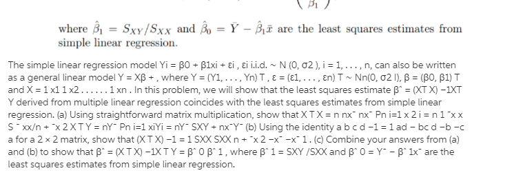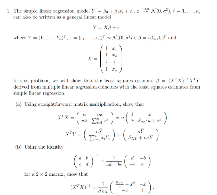


@ help here please
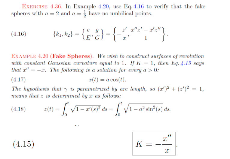
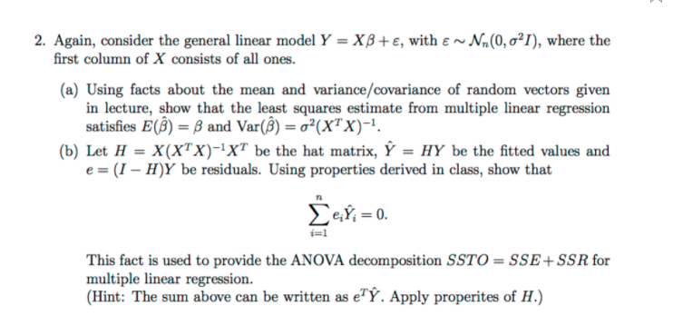
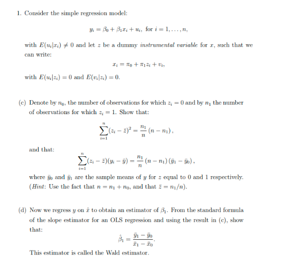
EXERCISE 4.36. In Example 4.20, use Eq. 4.16 to verify that the fake spheres with a = 2 and a = , have no umbilical points. (4.16) T. EXAMPLE 4.20 (Fake Spheres). We wish to construct surfaces of revolution with constant Gaussian curvature equal to 1. If K = 1, then Eq. 4.15 says that x" = -x. The following is a solution for every a > 0: (4.17) x(t) = a cos(t). The hypothesis that y is parametrizationgth, so (x')2 + (2')2 = 1, means that z is determined by x as follows: (4.18) = (t) = VI - x'(s)2 ds = 1 - a2 sin? (s) ds. (4.15) K1. Consider the simple regression model: V/i = Po+ Piri +ui, for i = 1, ..., n, with E(ur,) 7 0 and let z be a dummy instrumental variable for a, such that we can write: with E(uilz;) = 0 and E(vilzi) = 0. (c) Denote by no, the number of observations for which z =0 and by n, the number of observations for which z, = 1. Show that: (a - 2) = =(n-m). 1=1 and that: [(8 -=)(3: - 9) = 7 "(n - ni) (31 - 90) . where to and g are the sample means of y for z equal to 0 and 1 respectively. (Hint: Use the fact that n = nj + no, and that = = m). (d) Now we regress y on i to obtain an estimator of 81. From the standard formula of the slope estimator for an OLS regression and using the result in (c), show that: By1 - 90 I1 - To This estimator is called the Wald estimator.2. Again, consider the general linear model Y = XB + , with & ~ Nn(0, o?/), where the first column of X consists of all ones. (a) Using facts about the mean and variance/covariance of random vectors given in lecture, show that the least squares estimate from multiple linear regression satisfies E(B) = B and Var(B) = ?(XTX)-1. (b) Let H = X(X X)-1XT be the hat matrix, Y = HY be the fitted values and e = (I - H)Y be residuals. Using properties derived in class, show that n Een = 0. i=1 This fact is used to provide the ANOVA decomposition SSTO = SSE + SSR for multiple linear regression. (Hint: The sum above can be written as e?Y. Apply properites of H.)\f1. The simple linear regression model Y, = Bo + Bir; +;, &; " N(0, 0'), i = 1, ..., n, can also be written as a general linear model Y = XB+E, where Y = (Y1, . . ., Yn), E = (61, . . . .E.)? ~ Na. (0, 621), B = (Bo, Bi) and T2 X = In In this problem, we will show that the least squares estimate B = (XTX)-1XTY derived from multiple linear regression coincides with the least squares estimates from simple linear regression. (a) Using straightforward matrix multiplication, show that XX= (ni _mix ) =n( x Smo+2) XTY = _ _X ) =(SxY + niY (b) Using the identity ( " * ) d ad - bc -c a for a 2 x 2 matrix, show that Sxx + 12 (x X)= -I SXX -T 1
