Help me with constraints, with the project!

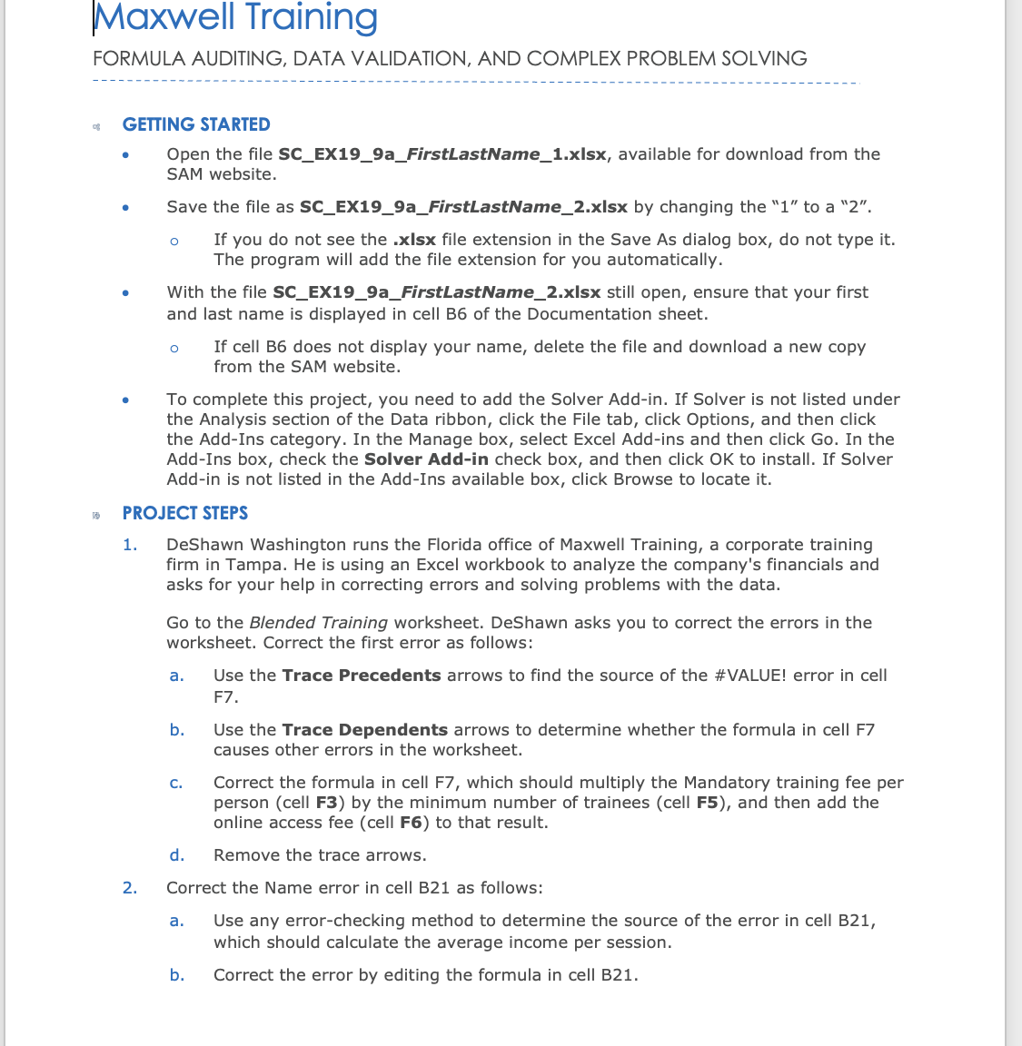
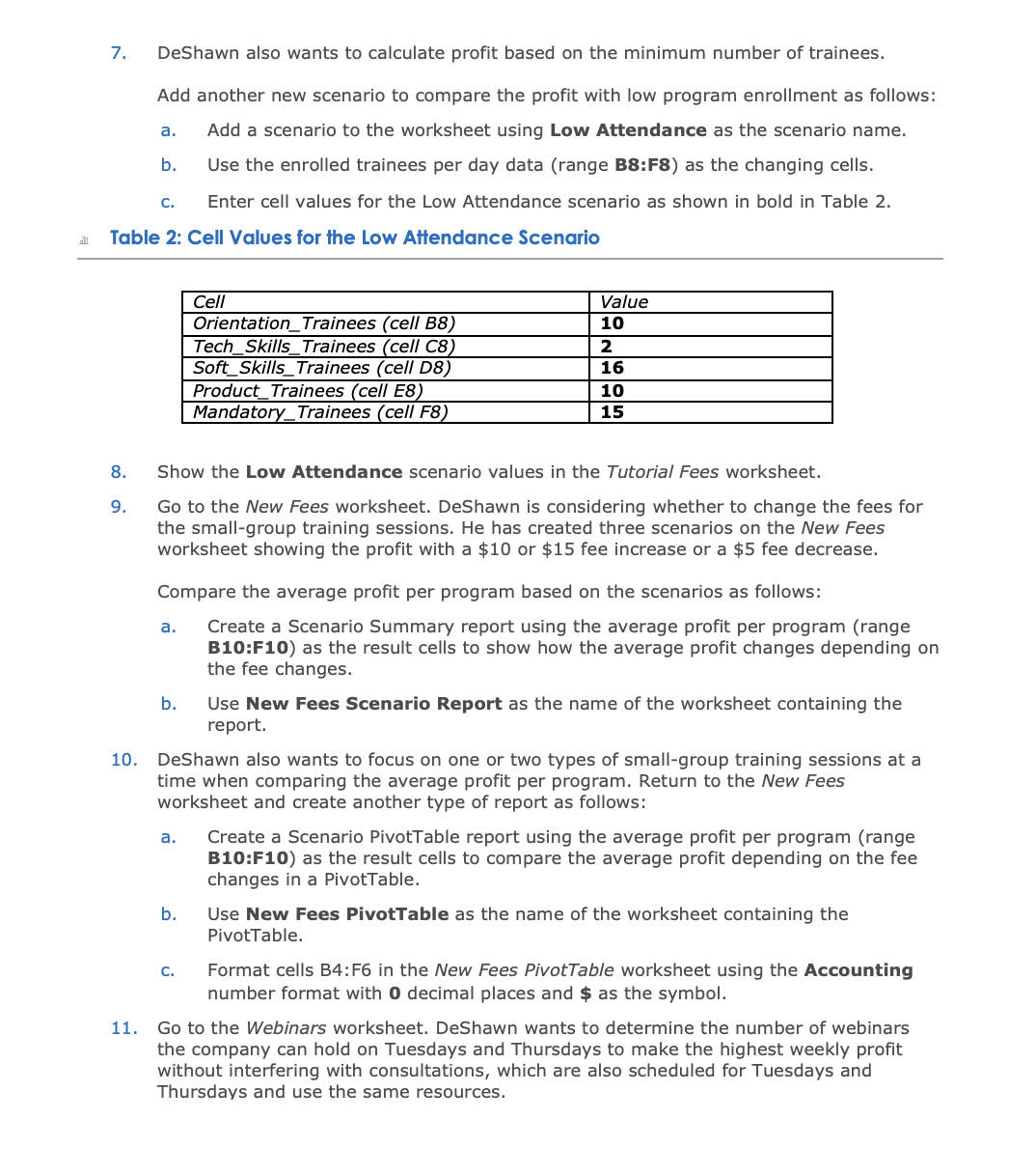FORMULA AUDITING, DATA VALIDATION, AND COMPLEX PROBLEM SOLVING a GETING STARTED - Open the file SC_EX19_9a_FirstLastName_1.xIsx, available for download from the SAM website. - Save the file as SC_EX19_9a_FirstLastName_2.xIsx by changing the "1" to a "2". - If you do not see the .xlsx file extension in the Save As dialog box, do not type it. The program will add the file extension for you automatically. - With the file SC_EX19_9a_FirstLastName_2.xIsx still open, ensure that your first and last name is displayed in cell B6 of the Documentation sheet. - If cell B6 does not display your name, delete the file and download a new copy from the SAM website. - To complete this project, you need to add the Solver Add-in. If Solver is not listed under the Analysis section of the Data ribbon, click the File tab, click Options, and then click the Add-Ins category. In the Manage box, select Excel Add-ins and then click Go. In the Add-Ins box, check the Solver Add-in check box, and then click OK to install. If Solver Add-in is not listed in the Add-Ins available box, click Browse to locate it. PROJECT STEPS 1. DeShawn Washington runs the Florida office of Maxwell Training, a corporate training firm in Tampa. He is using an Excel workbook to analyze the company's financials and asks for your help in correcting errors and solving problems with the data. Go to the Blended Training worksheet. DeShawn asks you to correct the errors in the worksheet. Correct the first error as follows: a. Use the Trace Precedents arrows to find the source of the \#VALUE! error in cell F7. b. Use the Trace Dependents arrows to determine whether the formula in cell F7 causes other errors in the worksheet. c. Correct the formula in cell F7, which should multiply the Mandatory training fee per person (cell F3) by the minimum number of trainees (cell F5), and then add the online access fee (cell F6) to that result. d. Remove the trace arrows. 2. Correct the Name error in cell B21 as follows: a. Use any error-checking method to determine the source of the error in cell B21, which should calculate the average income per session. b. Correct the error by editing the formula in cell B21. Use Solver to find this information as follows: a. Use the total weekly profit (cell G16, named Total_Weekly_Profit) as the objective cell in the Solver model, with the goal of determining the maximum value for that cell. b. Use the number of Tuesday and Thursday sessions for the five programs (range B4:F5) as the changing variable cells. c. Determine and enter the constraints based on the information provided in Table 3. d. Use Simplex LP as the solving method to find a global optimal solution. e. Save the Solver model in cell A26. f. Solve the model, keeping the Solver solution. Table 3: Solver Constraints 12. DeShawn wants to document the answer Solver found, including the constraints and a list of the values Solver changed to solve the problem. Produce an Answer report for the Solver model as follows: a. Solve the model again, this time choosing to produce an Answer report. b. Use Webinar Answer Report as the name of the worksheet containing the Answer report. our workbook should look like the Final Figures on the following pages. Save your changes, lose the workbook, and then exit Excel. Follow the directions on the SAM website to submit your ompleted project. 3. Correct the divide-by-zero errors as follows: a. Evaluate the formula in cell B17 to determine which cell is causing the divide-byzero error. b. Correct the formula in cell B17, which should divide the income per program (cell B15) by the minimum number of trainees (cell B5). c. Fill the range C17:F17 with the formula in cell B17. (Hint: You will correct the new error in cell C17 in the following steps.) 4. DeShawn suspects that the two remaining errors are related to the zero value in cell C5. He wants to make sure that anyone entering the minimum number of trainees enters a number greater than zero. Add data validation to the range B5:F5 as follows: a. Set a data validation rule for the range B5:F5 that allows only whole number values greater than 0. b. Add an Input Message using Number of Trainees as the Input Message title and the following text as the Input message: Enter the minimum number of trainees for this program. c. Add an Error Alert using the Stop style, Trainees Error as the Error Alert title, and the following text as the Error message: The minimum number of trainees must be greater than 0 . 5. Identify the invalid data in the worksheet and correct the entry as follows: a. Circle the invalid data in the worksheet. b. Type 15 as the minimum number of trainees for the Tech Skills program (cell C5). c. Verify that this change cleared the remaining errors in the worksheet. 6. Go to the Tutorial Fees worksheet. This worksheet analyzes financial data for smallgroup training sessions, which Maxwell Training runs throughout the day. DeShawn has already created a scenario named Current Enrollment that calculates profit based on the current number of trainees enrolled for each program. He also wants to calculate profit based on the maximum number of trainees. Add a new scenario to compare the profit with maximum enrollments as follows: a. Use Max Attendance as the scenario name. b. Use the enrolled trainees per day data (range B8:F8) as the changing cells. c. Enter cell values for the Max Attendance scenario as shown in bold in Table 1, which are the same values as in the range B7:F7. Table 1: Cell Values for the Max Attendance Scenario 7. DeShawn also wants to calculate profit based on the minimum number of trainees. Add another new scenario to compare the profit with low program enrollment as follows: a. Add a scenario to the worksheet using Low Attendance as the scenario name. b. Use the enrolled trainees per day data (range B8:F8) as the changing cells. c. Enter cell values for the Low Attendance scenario as shown in bold in Table 2. Table 2: Cell Values for the Low Attendance Scenario 8. Show the Low Attendance scenario values in the Tutorial Fees worksheet. 9. Go to the New Fees worksheet. DeShawn is considering whether to change the fees for the small-group training sessions. He has created three scenarios on the New Fees worksheet showing the profit with a $10 or $15 fee increase or a $5 fee decrease. Compare the average profit per program based on the scenarios as follows: a. Create a Scenario Summary report using the average profit per program (range B10:F10) as the result cells to show how the average profit changes depending on the fee changes. b. Use New Fees Scenario Report as the name of the worksheet containing the report. 10. DeShawn also wants to focus on one or two types of small-group training sessions at a time when comparing the average profit per program. Return to the New Fees worksheet and create another type of report as follows: a. Create a Scenario PivotTable report using the average profit per program (range B10:F10) as the result cells to compare the average profit depending on the fee changes in a PivotTable. b. Use New Fees PivotTable as the name of the worksheet containing the PivotTable. c. Format cells B4:F6 in the New Fees PivotTable worksheet using the Accounting number format with 0 decimal places and $ as the symbol. 11. Go to the Webinars worksheet. DeShawn wants to determine the number of webinars the company can hold on Tuesdays and Thursdays to make the highest weekly profit without interfering with consultations, which are also scheduled for Tuesdays and Thursdays and use the same resources. FORMULA AUDITING, DATA VALIDATION, AND COMPLEX PROBLEM SOLVING a GETING STARTED - Open the file SC_EX19_9a_FirstLastName_1.xIsx, available for download from the SAM website. - Save the file as SC_EX19_9a_FirstLastName_2.xIsx by changing the "1" to a "2". - If you do not see the .xlsx file extension in the Save As dialog box, do not type it. The program will add the file extension for you automatically. - With the file SC_EX19_9a_FirstLastName_2.xIsx still open, ensure that your first and last name is displayed in cell B6 of the Documentation sheet. - If cell B6 does not display your name, delete the file and download a new copy from the SAM website. - To complete this project, you need to add the Solver Add-in. If Solver is not listed under the Analysis section of the Data ribbon, click the File tab, click Options, and then click the Add-Ins category. In the Manage box, select Excel Add-ins and then click Go. In the Add-Ins box, check the Solver Add-in check box, and then click OK to install. If Solver Add-in is not listed in the Add-Ins available box, click Browse to locate it. PROJECT STEPS 1. DeShawn Washington runs the Florida office of Maxwell Training, a corporate training firm in Tampa. He is using an Excel workbook to analyze the company's financials and asks for your help in correcting errors and solving problems with the data. Go to the Blended Training worksheet. DeShawn asks you to correct the errors in the worksheet. Correct the first error as follows: a. Use the Trace Precedents arrows to find the source of the \#VALUE! error in cell F7. b. Use the Trace Dependents arrows to determine whether the formula in cell F7 causes other errors in the worksheet. c. Correct the formula in cell F7, which should multiply the Mandatory training fee per person (cell F3) by the minimum number of trainees (cell F5), and then add the online access fee (cell F6) to that result. d. Remove the trace arrows. 2. Correct the Name error in cell B21 as follows: a. Use any error-checking method to determine the source of the error in cell B21, which should calculate the average income per session. b. Correct the error by editing the formula in cell B21. Use Solver to find this information as follows: a. Use the total weekly profit (cell G16, named Total_Weekly_Profit) as the objective cell in the Solver model, with the goal of determining the maximum value for that cell. b. Use the number of Tuesday and Thursday sessions for the five programs (range B4:F5) as the changing variable cells. c. Determine and enter the constraints based on the information provided in Table 3. d. Use Simplex LP as the solving method to find a global optimal solution. e. Save the Solver model in cell A26. f. Solve the model, keeping the Solver solution. Table 3: Solver Constraints 12. DeShawn wants to document the answer Solver found, including the constraints and a list of the values Solver changed to solve the problem. Produce an Answer report for the Solver model as follows: a. Solve the model again, this time choosing to produce an Answer report. b. Use Webinar Answer Report as the name of the worksheet containing the Answer report. our workbook should look like the Final Figures on the following pages. Save your changes, lose the workbook, and then exit Excel. Follow the directions on the SAM website to submit your ompleted project. 3. Correct the divide-by-zero errors as follows: a. Evaluate the formula in cell B17 to determine which cell is causing the divide-byzero error. b. Correct the formula in cell B17, which should divide the income per program (cell B15) by the minimum number of trainees (cell B5). c. Fill the range C17:F17 with the formula in cell B17. (Hint: You will correct the new error in cell C17 in the following steps.) 4. DeShawn suspects that the two remaining errors are related to the zero value in cell C5. He wants to make sure that anyone entering the minimum number of trainees enters a number greater than zero. Add data validation to the range B5:F5 as follows: a. Set a data validation rule for the range B5:F5 that allows only whole number values greater than 0. b. Add an Input Message using Number of Trainees as the Input Message title and the following text as the Input message: Enter the minimum number of trainees for this program. c. Add an Error Alert using the Stop style, Trainees Error as the Error Alert title, and the following text as the Error message: The minimum number of trainees must be greater than 0 . 5. Identify the invalid data in the worksheet and correct the entry as follows: a. Circle the invalid data in the worksheet. b. Type 15 as the minimum number of trainees for the Tech Skills program (cell C5). c. Verify that this change cleared the remaining errors in the worksheet. 6. Go to the Tutorial Fees worksheet. This worksheet analyzes financial data for smallgroup training sessions, which Maxwell Training runs throughout the day. DeShawn has already created a scenario named Current Enrollment that calculates profit based on the current number of trainees enrolled for each program. He also wants to calculate profit based on the maximum number of trainees. Add a new scenario to compare the profit with maximum enrollments as follows: a. Use Max Attendance as the scenario name. b. Use the enrolled trainees per day data (range B8:F8) as the changing cells. c. Enter cell values for the Max Attendance scenario as shown in bold in Table 1, which are the same values as in the range B7:F7. Table 1: Cell Values for the Max Attendance Scenario 7. DeShawn also wants to calculate profit based on the minimum number of trainees. Add another new scenario to compare the profit with low program enrollment as follows: a. Add a scenario to the worksheet using Low Attendance as the scenario name. b. Use the enrolled trainees per day data (range B8:F8) as the changing cells. c. Enter cell values for the Low Attendance scenario as shown in bold in Table 2. Table 2: Cell Values for the Low Attendance Scenario 8. Show the Low Attendance scenario values in the Tutorial Fees worksheet. 9. Go to the New Fees worksheet. DeShawn is considering whether to change the fees for the small-group training sessions. He has created three scenarios on the New Fees worksheet showing the profit with a $10 or $15 fee increase or a $5 fee decrease. Compare the average profit per program based on the scenarios as follows: a. Create a Scenario Summary report using the average profit per program (range B10:F10) as the result cells to show how the average profit changes depending on the fee changes. b. Use New Fees Scenario Report as the name of the worksheet containing the report. 10. DeShawn also wants to focus on one or two types of small-group training sessions at a time when comparing the average profit per program. Return to the New Fees worksheet and create another type of report as follows: a. Create a Scenario PivotTable report using the average profit per program (range B10:F10) as the result cells to compare the average profit depending on the fee changes in a PivotTable. b. Use New Fees PivotTable as the name of the worksheet containing the PivotTable. c. Format cells B4:F6 in the New Fees PivotTable worksheet using the Accounting number format with 0 decimal places and $ as the symbol. 11. Go to the Webinars worksheet. DeShawn wants to determine the number of webinars the company can hold on Tuesdays and Thursdays to make the highest weekly profit without interfering with consultations, which are also scheduled for Tuesdays and Thursdays and use the same resources