Answered step by step
Verified Expert Solution
Question
1 Approved Answer
hey can you please help me with the DATA (from instructions) requirement 6 and the graph information? Analysis 2 Using Excel for Cost-Volume-Profit (CVP) Analysis
hey can you please help me with the DATA (from instructions)
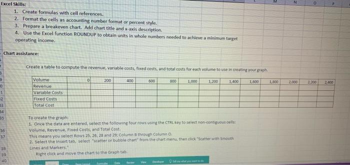
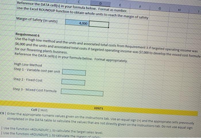
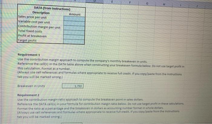
Analysis 2 Using Excel for Cost-Volume-Profit (CVP) Analysis 3 The Oceanside Garden Nursery buys flowering plants in four-inch pots for $1.50 each and sells them for $3.00 4 each. Management budgets monthly fixed costs of $2,600 for sales volumes between 0 and 7,500 plants. 5 Use the blue shaded areas on the ENTERANSWERS tab for inputs. Always use cell references and formulas where appropriate to receive full credit. If you copy/paste from the Instructions tab you will 6 be marked wrong, NO 12 8 9 Requirements: 10 1. Use the contribution margin approach to compute the company's monthly breakeven point in units. 11 2. Use the contribution margin ratio approach to compute the breakeven point in sales dollars. 3. Use the contribution margin approach to compute the monthly sales tevel (in units) required to earn a target operating income of $6,000. 4. Use the contribution margin approach to compute the monthly sales level (in units) required to earn a 13 target operating Income of $6,000 5. Use the contribution margin approach to compute the margin of safety (in units) using the target operating income of $6,000. 6. Use the high low method and the units and associated total costs from Requirement 3 if targeted operating income was $6,000 and the units and associated total costs If targeted operating income was $7,000 to develop the mixed cost formula for our flowering plants business 7. Prepare a graph of the company's CVP relationships. Include the sales revenue line, the fixed cost line, and the total cost line by completing the table below. Create a chart title and label the axes. 14 15 10 M N N o Excel Skills: 1. Create formulas with cell references. 2. Format the cells as accounting number format or percent style. 3. Prepare a breakeven chart. Add chart title and x-axis description 4. Use the Excel function ROUNDUP to obtain units in whole numbers needed to achieve a minimum target operating Income. Chart assistance: Create a table to compute the revenue, variable costs, fixed costs, and total costs for each volume use in creating your graph. 0 200 400 000 800 1,000 1.200 1.400 1,600 1,800 2.000 2200 2.400 1 -2 39 Volume Revenue Variable Costs Fixed Costs Total Cost 36 37 To create the graph: 1. Once the data are entered, select the following four rows using the CTRL key to select non-contiguous cells: Volume, Revenue, Fixed Costs, and Total Cost. This means you select Rows 25, 26, 28 and 29: Column through Columno 2. Select the Insert tab, select "scatter-or bubble chart" from the chart menu, then clickscatter with Smooth Lines and Markers, Right click and move the chart to the Graph tab 30 ao 40 are De D E F Reference the DATA cell(s) in your formula below. Format as number. Use the Excel ROUNDUP function to obtain whole units to reach the margin of safety G H Margin of Safety (in units) 4,000 Requirement 6 Use the high low method and the units and associated total costs from Requirement 3 if targeted operating income was $6,000 and the units and associated total costs if targeted operating income was $7,000 to develop the mixed cost formula for our flowering plants business. Reference the DATA cell(s) in your formula below. Format appropriately. High Low Method Step 1 - Variable cost per unit Step 2 - Fixed Cost Step 3 - Mixed Cost Formula HINTS Cell Hint: 09 | Enter the appropriate numeric values given on the Instructions tab. Use an equal sign (=) and the appropriate cells previously completed in the DATA table to calculate the values that are not directly given on the instructions tab. Do not use equal sign Use the function =ROUNDUPL), to calculate the target sales level. Use the function =ROUNDUP(), to calculate the marrin nfcom E F G DATA (from instructions) Description Amount Sales price per unit Variable cost per unit Contribution margin per unit Total fixed costs Profit at breakeven Target profit Requirement 1 Use the contribution margin approach to compute the company's monthly breakeven in units. Reference the cell(s) in the DATA table above when constructing your breakeven formula below. Do not use target profit in this calculation. Format as a number. (Always use cell references and formulas where appropriate to receive full credit. If you copy/paste from the Instructions tab you will be marked wrong.) Breakeven in Units 1.733 Requirement 2 Use the contribution margin ratio approach to compute the breakeven point in sales dollars. Reference the DATA cell(s) in your formula for contribution margin ratio below. Do not use target profit in these calculations Format the ratio as a percentage and the breakeven in dollars as accounting number format in whole dollars. (Always use cell references and formulas where appropriate to receive full credit. If you copy/paste from the instructions tab you will be marked wrong.) requirement 6 and the graph information? 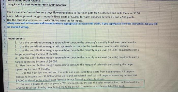


Step by Step Solution
There are 3 Steps involved in it
Step: 1

Get Instant Access to Expert-Tailored Solutions
See step-by-step solutions with expert insights and AI powered tools for academic success
Step: 2

Step: 3

Ace Your Homework with AI
Get the answers you need in no time with our AI-driven, step-by-step assistance
Get Started


