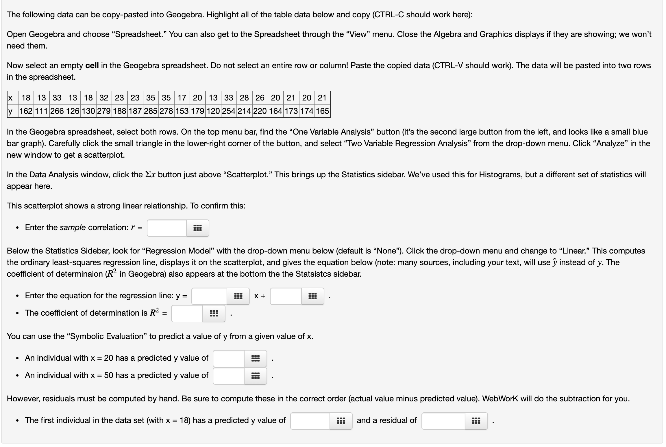
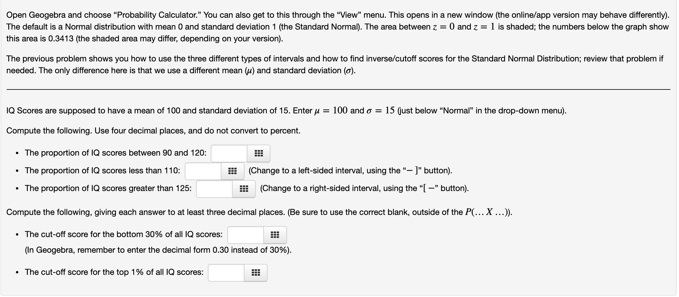
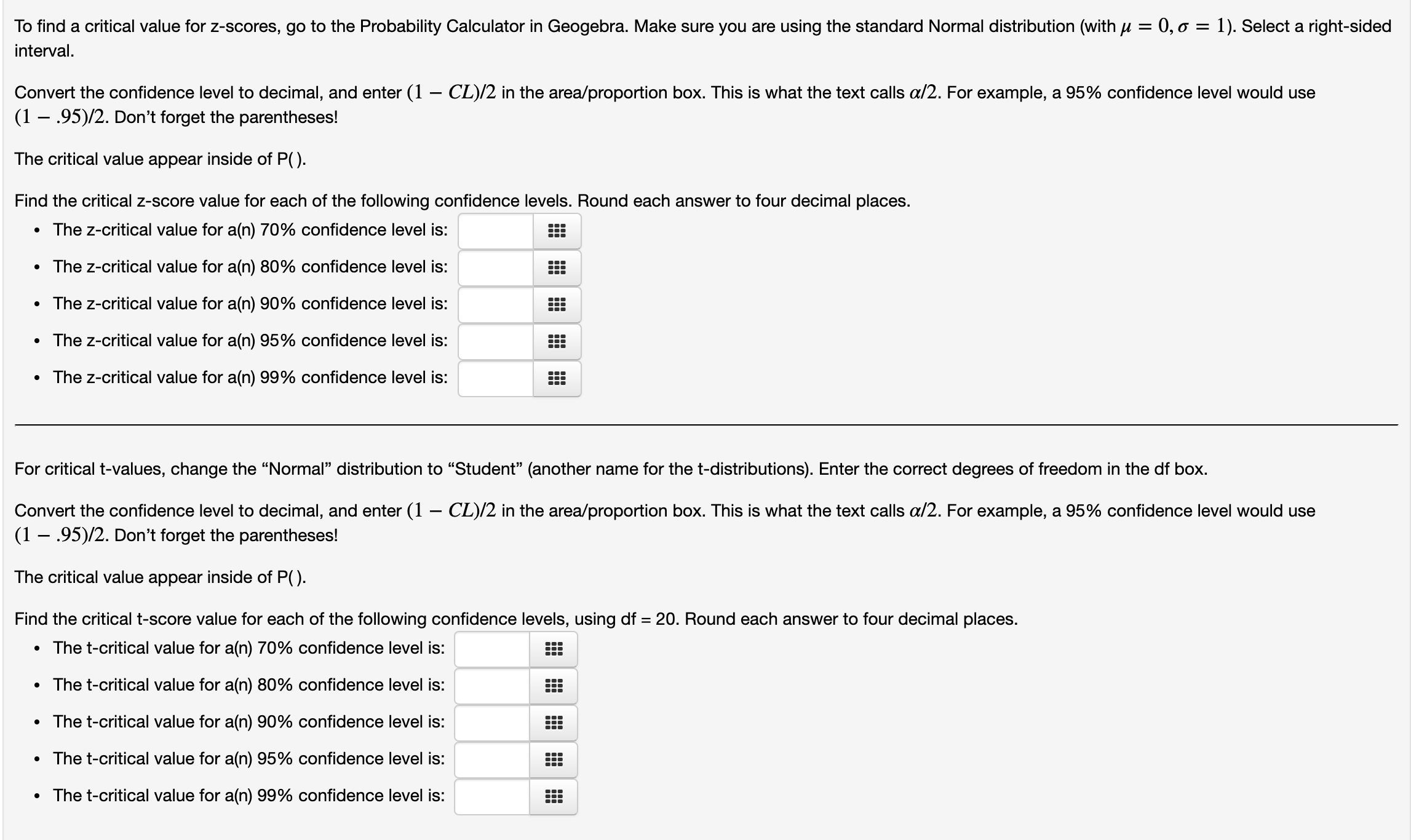
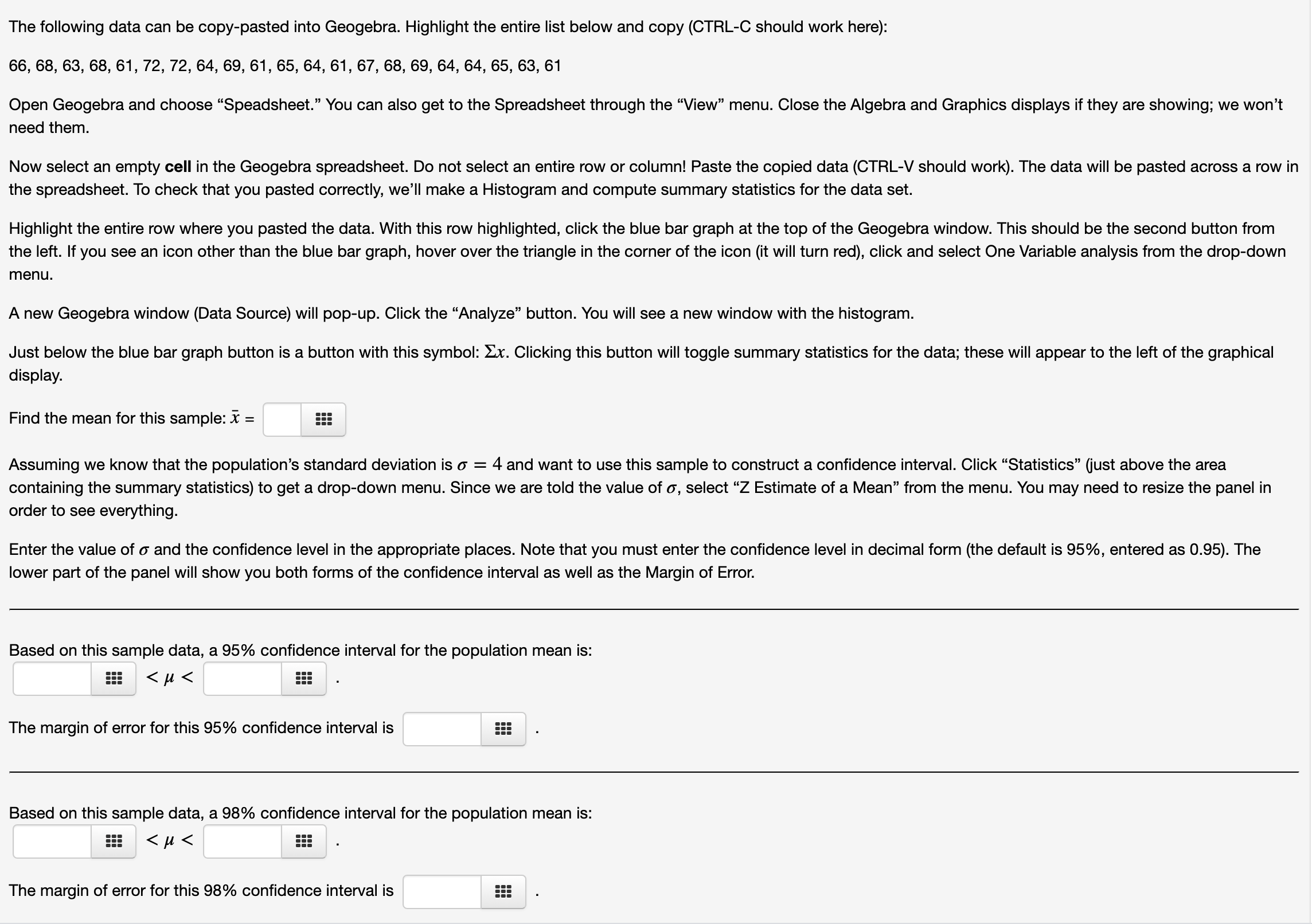
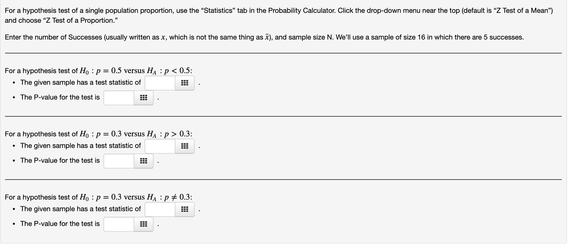
Hi, can someone help me with these questions?

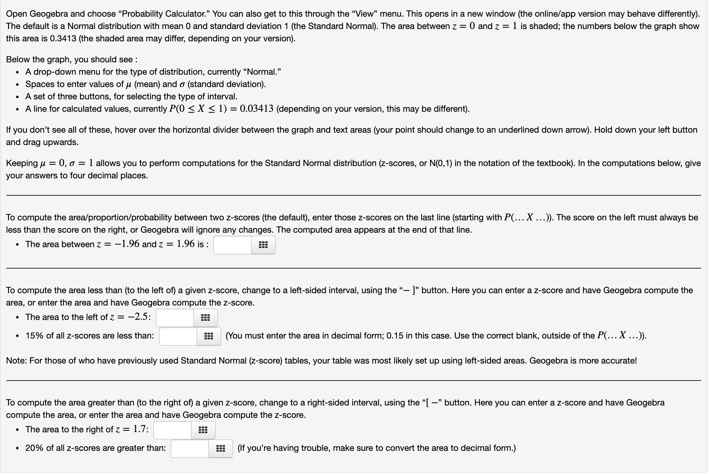
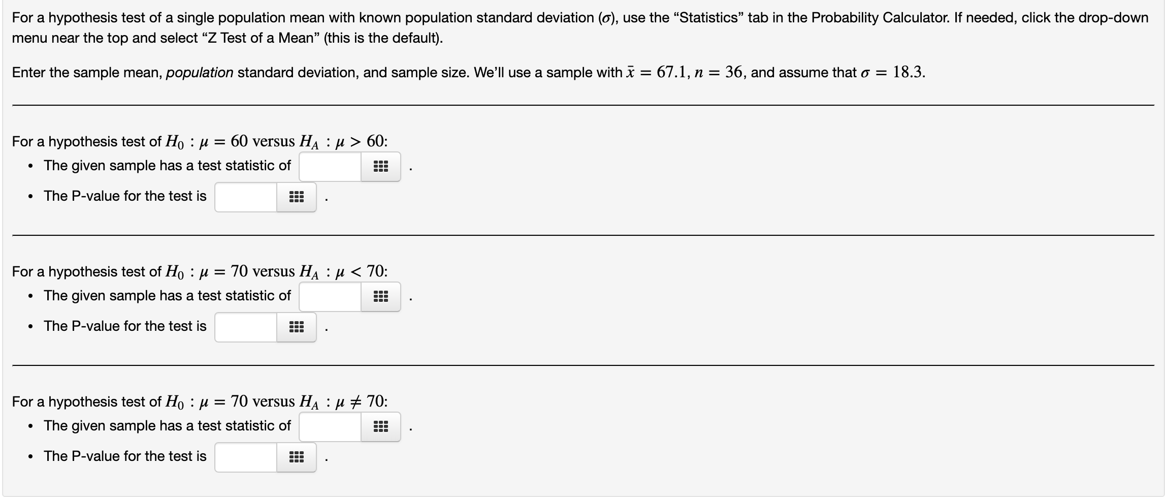
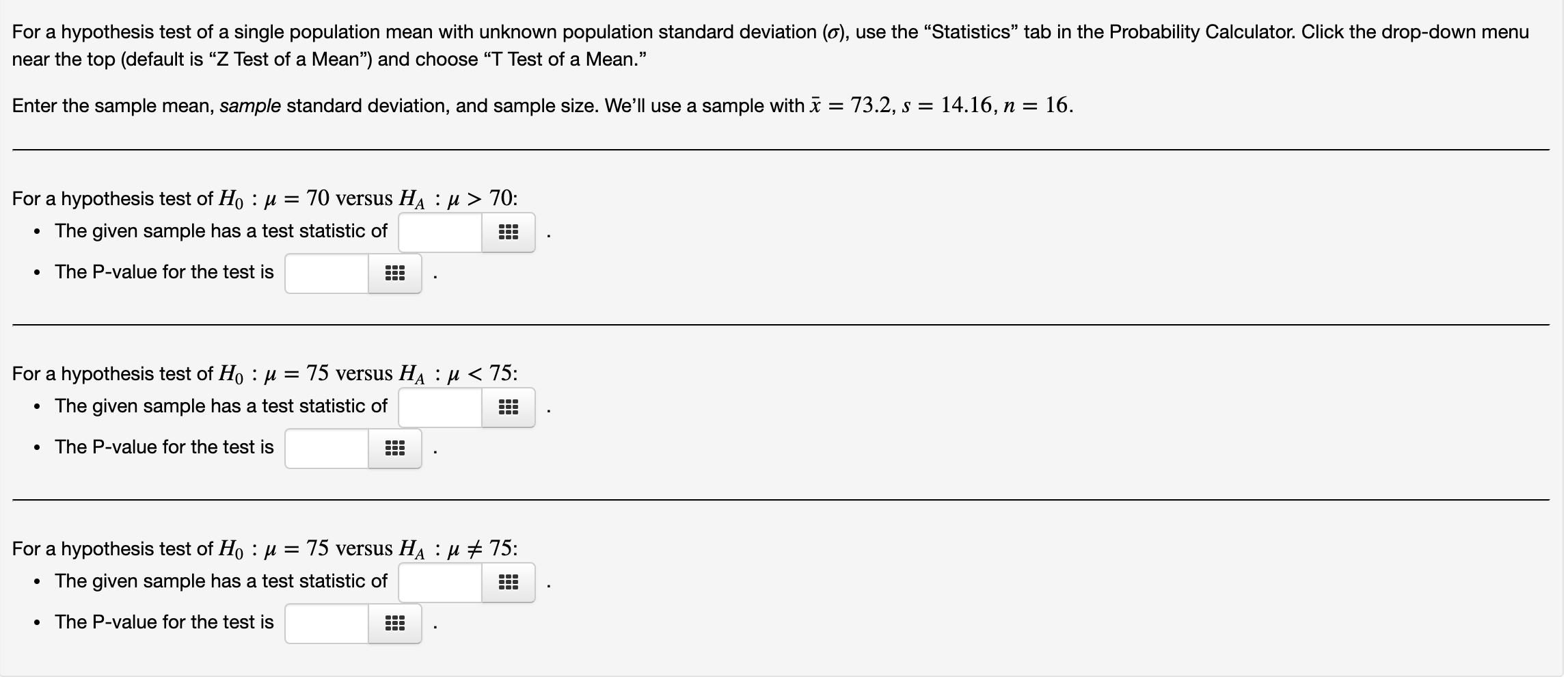
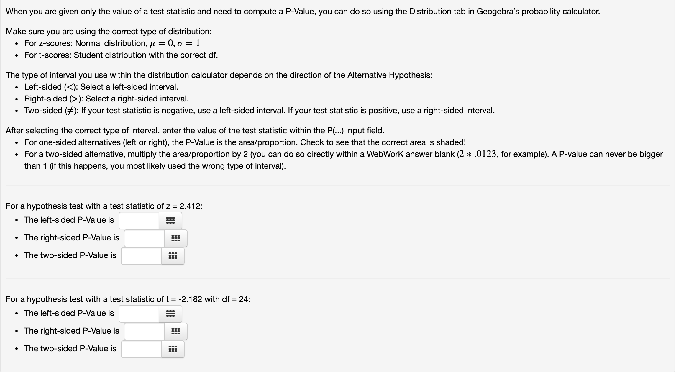
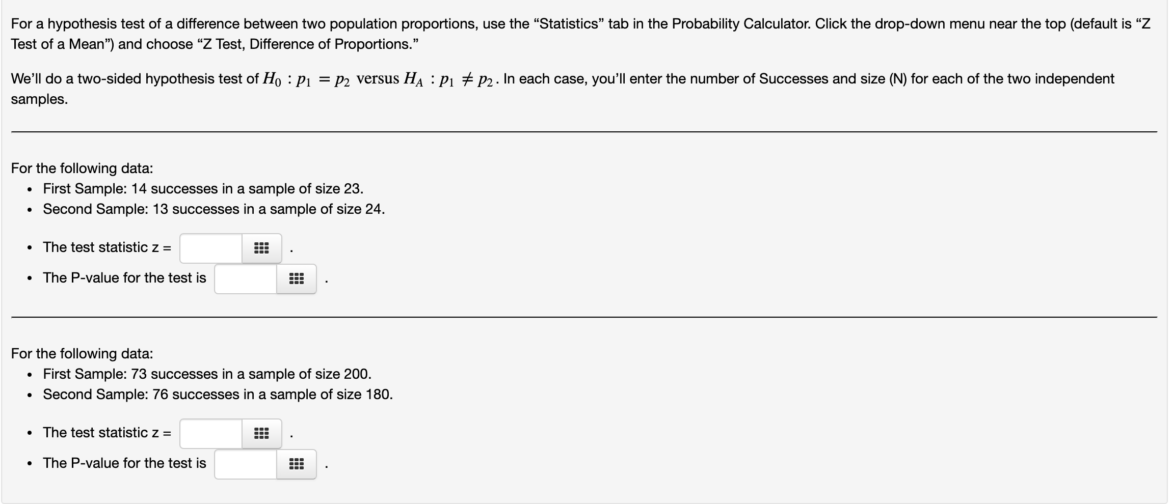
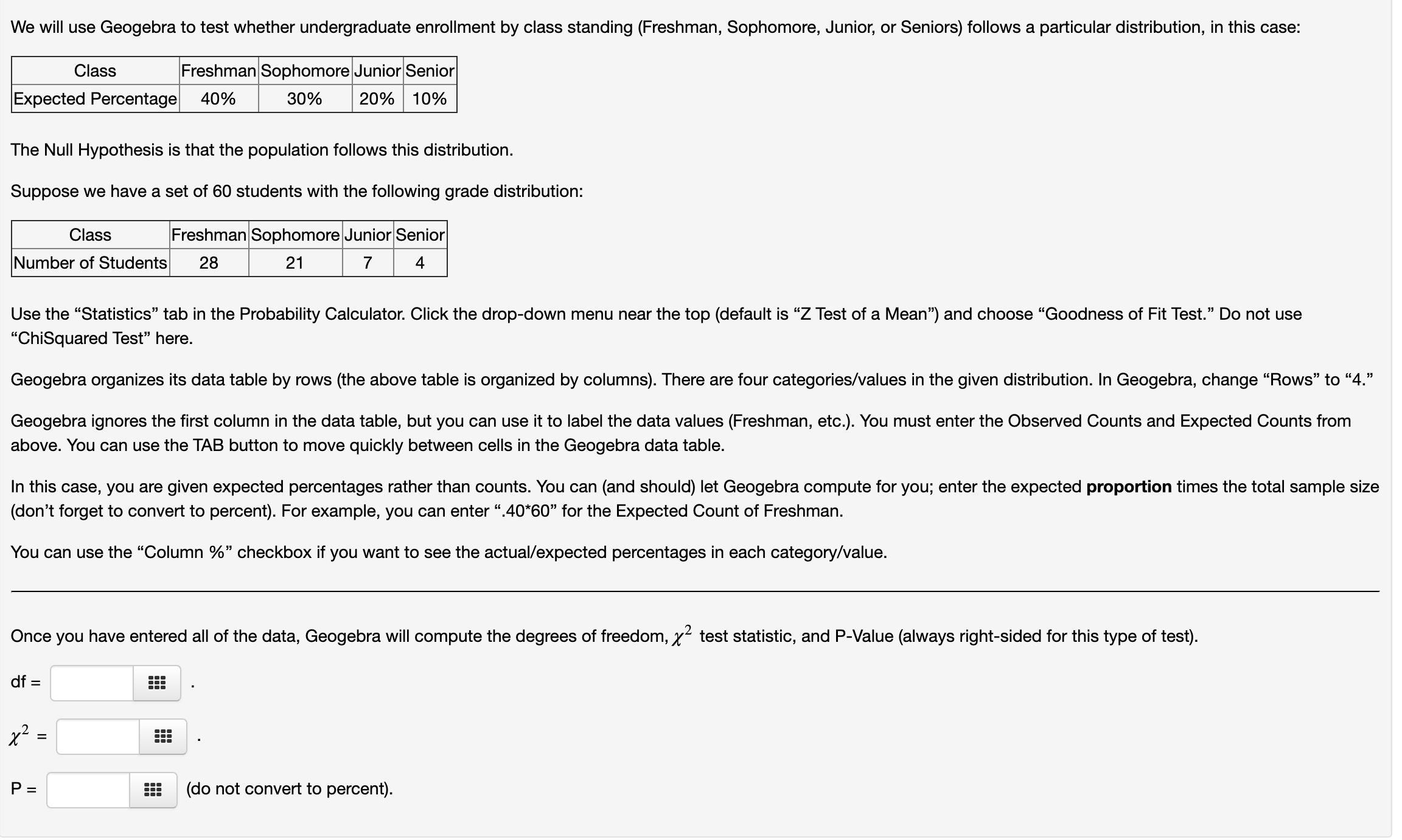
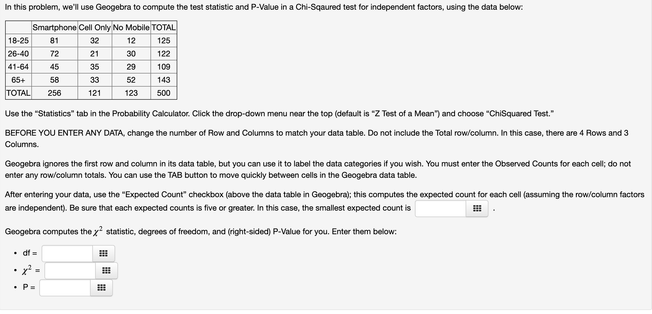
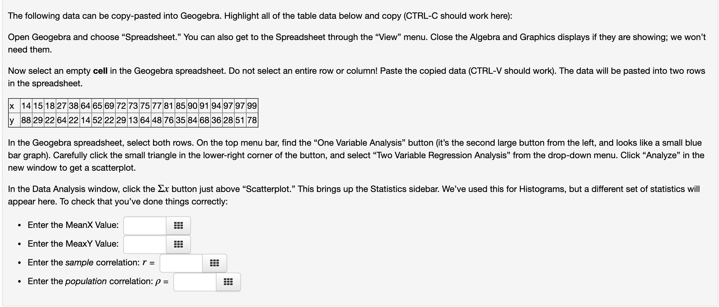
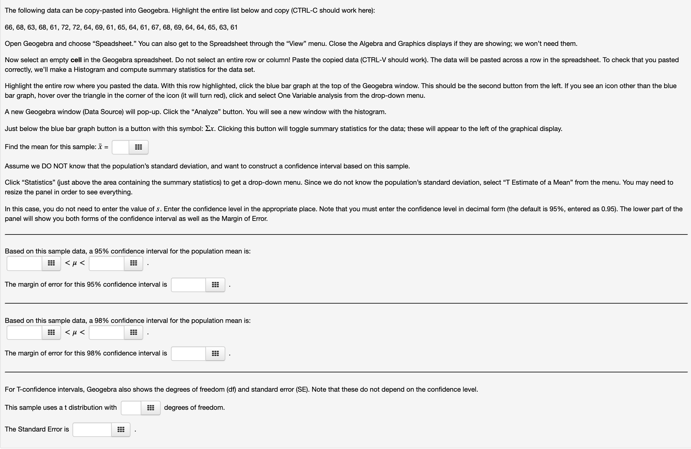
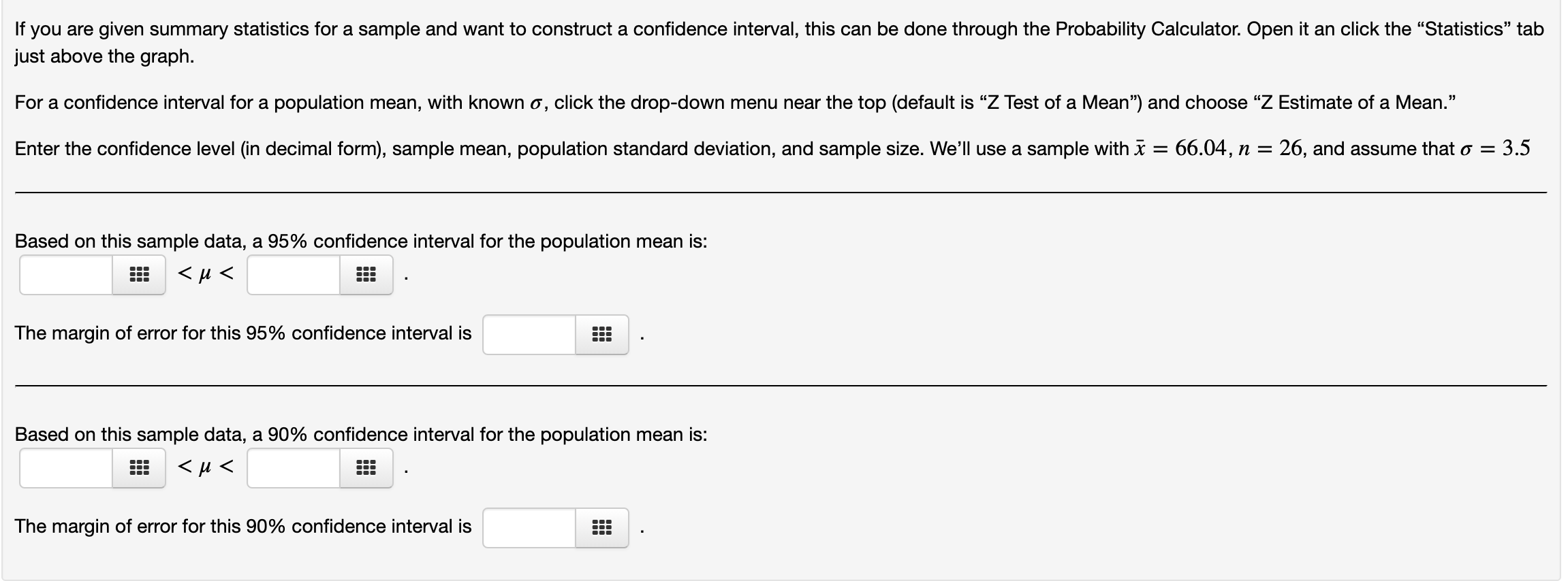
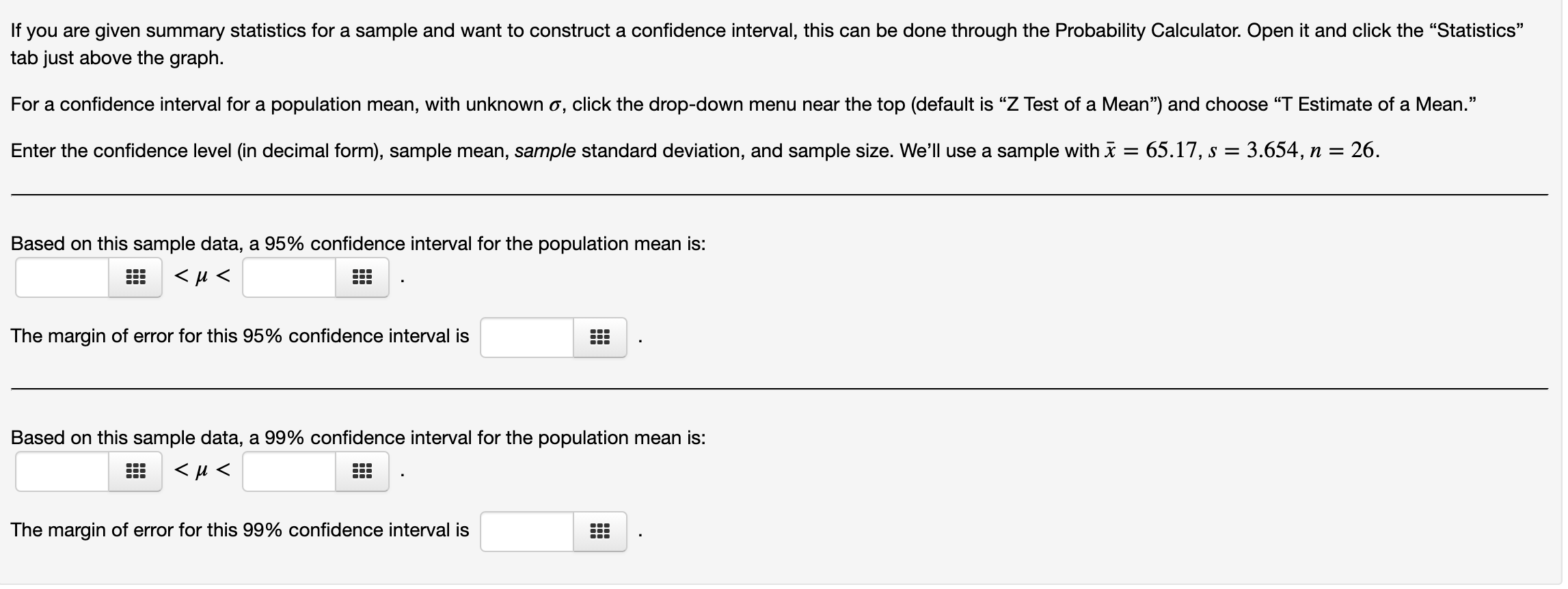
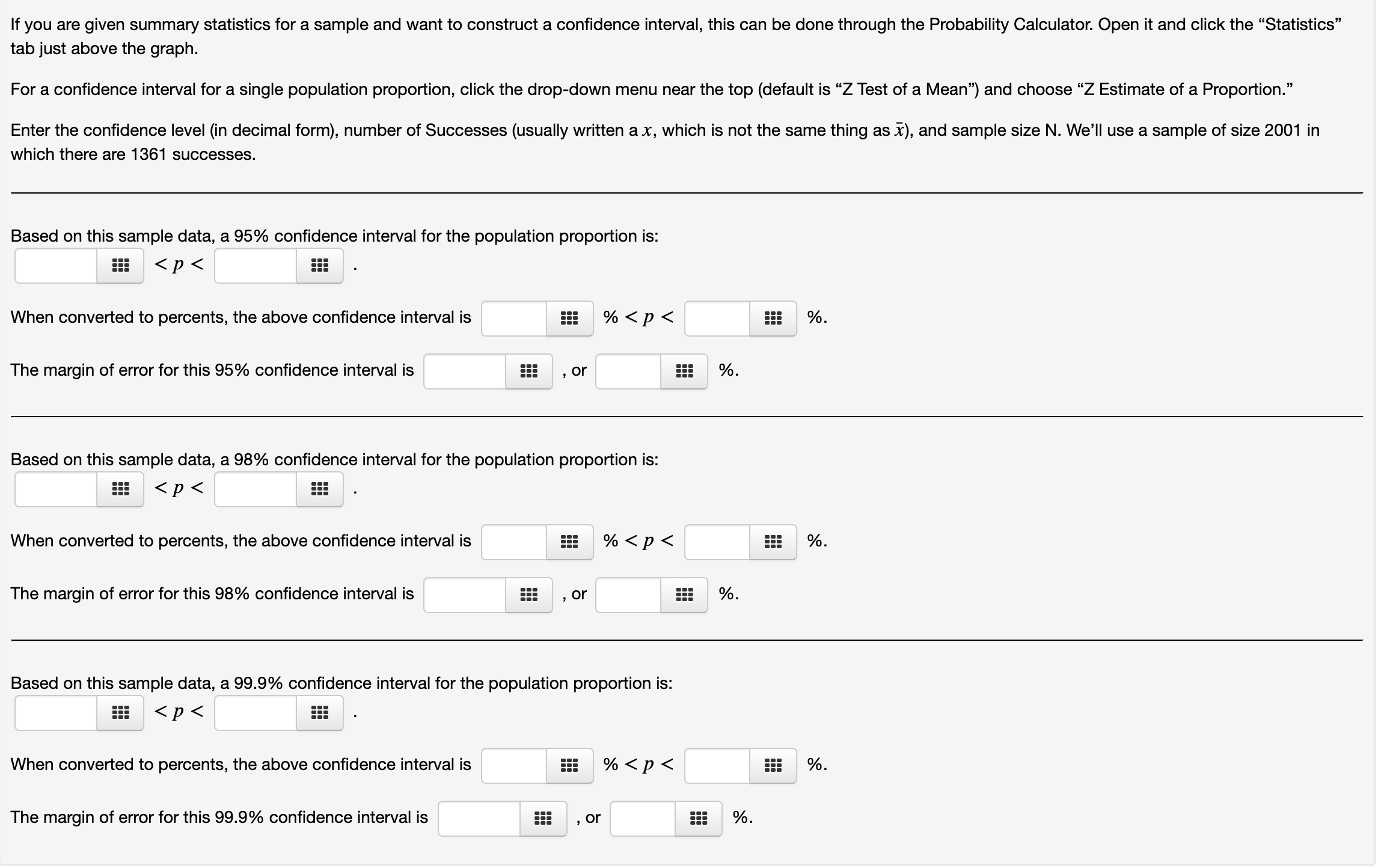
Open Geogebra and choose "Probability Calculator.\" You can also get to this through the \"\\ew" menu. This opens in a new window (the online/app version may behave differently). The default is a Normal distribution with mean 0 and standard deviation 1 (the Standard Normal). The area between z = 0 and z = 1 is shaded; the numbers below the graph show this area is 0.3413 (the shaded area may differ, depending on your version). Below the graph, you should see : - A drop-down menu for the type of distribution, currently \"Normal." - Spaces to enter values of [4 (mean) and a (standard deviation). . A set of three buttons, for selecting the type of interval. . A line for calculated values, currently P(O S X S 1) = 0.03413 (depending on your version, this may be different). If you don't see all of these, hover over the horizontal divider between the graph and text areas (your point should change to an underlined down arrow). Hold down your left button and drag upwards. Keeping [4 = 0, a = 1 allows you to perform computations for the Standard Normal distribution (z-scores, or N(0,1) in the notation of the textbook). In the computations below, give your answers to four decimal places. To compute the area/proportion/probability between two zscores (the default), enter those z-scores on the last line (starting with P(. . . X . . .)). The score on the left must always be less than the score on the right, or Geogebra will ignore any changes. The computed area appears at the end of that line. - The area between 2 = l.96 and z = 1.96 is : To compute the area less than (to the left of) a given z-score, change to a left-sided interval, using the " ]" button. Here you can enter a z-score and have Geogebra compute the area, or enter the area and have Geogebra compute the z-score. - The area to the left of z = 2.5: - 15% of all z-scores are less than: (You must enter the area in decimal form; 0.15 in this case. Use the correct blank, outside of the P(. .. X ...)). Note: For those of who have previously used Standard Normal (z-score) tables, your table was most likely set up using left-sided areas. Geogebra is more accurate! To compute the area greater than (to the right of) a given z-score, change to a right-sided interval, using the \"[ \" button. Here you can enter a z-score and have Geogebra compute the area, or enter the area and have Geogebra compute the z-score. - The area to the right of z = 1.7: ' ESE - 20% of all z-scores are greater than: 525 (If you're having trouble, make sure to convert the area to decimal form.) For a hypothesis test of a single population mean with known population standard deviation (0'), use the "Statistics\" tab in the Probability Calculator. If needed, click the drop-down menu near the top and select \"Z Test of a Mean" (this is the default). Enter the sample mean, population standard deviation, and sample size. We'll use a sample with i = 67.1, n = 36, and assume that a' = 18.3. For a hypothesis test of Ho : p = 60 versus HA : u > 60: - The given sample has a test statistic of - The P-value for the test is : For a hypothesis test of Ho : ,u = 70 versus HA : ,u 70: - The given sample has a test statistic of ... . The P-value for the test is For a hypothesis test of H0 : u = 75 versus HA : [4 ): Select a right-sided interval. . Two-sided (#): If your test statistic is negative, use a left-sided interval. If your test statistic is positive, use a right-sided interval. After selecting the correct type of interval, enter the value of the test statistic within the P(...) input field. . For one-sided alternatives (left or right), the P-Value is the area/proportion. Check to see that the correct area is shaded! . For a two-sided alternative, multiply the area/proportion by 2 (you can do so directly within a WebWork answer blank (2 * .0123, for example). A P-value can never be bigger than 1 (if this happens, you most likely used the wrong type of interval). For a hypothesis test with a test statistic of z = 2.412: . The left-sided P-Value is . The right-sided P-Value is . The two-sided P-Value is For a hypothesis test with a test statistic of t = -2.182 with df = 24: . The left-sided P-Value is . The right-sided P-Value is . The two-sided P-Value isFor a hypothesis test of a difference between two population proportions, use the \"Statistics\" tab in the Probability Calculator. Click the drop-down menu near the top (default is "Z Test of a Mean") and choose \"Z Test, Difference of Proportions.\" We'll do a two-sided hypothesis test of Ho : p1 = 112 versus HA : p1 a p2. In each case, you'll enter the number of Successes and size (N) for each of the two independent samples. For the following data: . First Sample: 14 successes in a sample of size 23. . Second Sample: 13 successes in a sample of size 24. - The test statistic z = SEE - The P-value for the test is For the following data: First Sample: 73 successes in a sample of size 200. Second Sample: 76 successes in a sample of size 180. The test statistic z = is The P-value for the test is ' ' :=: For a hypothesis test of a difference between two population means, use the "Statistics" tab in the Probability Calculator. Click the drop-down menu near the top (default is "Z Test of a Mean\") and choose \"T Test, Difference of Means.\" We'll do a right-sided hypothesis test of H0 : m = ['2 versus HA : [41 > #2; select the correct Alternative Hypotheis in Geogebra. Make sure that the \"Pooled\" box is not selected. Enter the mean (3c), sample standard deviation (5), and size (N) for each of the two independent samples. For the following sample data: . First Sample: Mean = 65.87, Standard Deviation = 16.29, Sample Size = 23. . Second Sample: Mean = 58.17, Standard Deviation = 12.34, Sample Size = 24. Use Geogebra to compute the following values; giving your results to at least three decimal places: . The value of the test statistic: t = ::: . The degrees of freedom: df = i :=: (do not convert to percent). . The P-value: ' We will use Geogebra to test whether undergraduate enrollment by class standing (Freshman, Sophomore, Junior, or Seniors) follows a particular distribution, in this case: Class Freshman Sophomore Junior Senior Expected Percentagel 40% 30% 20% | 10% The Null Hypothesis is that the population follows this distribution. Suppose we have a set of 60 students with the following grade distribution: Class Freshman Sophomore Junior Senior Number of Students 28 I 21 I 7 4 Use the \"Statistics\" tab in the Probability Calculator. Click the drop-down menu near the top (default is \"Z Test of a Mean") and choose \"Goodness of Fit Test." Do not use \"ChiSquared Test\" here. Geogebra organizes its data table by rows (the above table is organized by columns). There are four categories/values in the given distribution. In Geogebra, change \"Rows" to \"4." Geogebra ignores the first column in the data table, but you can use it to label the data values (Freshman, etc.). You must enter the Observed Counts and Expected Counts from above. You can use the TAB button to move quickly between cells in the Geogebra data table. In this case, you are given expected percentages rather than counts. You can (and should) let Geogebra compute for you; enter the expected proportion times the total sample size (don't forget to convert to percent). For example, you can enter ".40'60\" for the Expected Count of Freshman. You can use the \"Column %\" checkbox if you want to see the actuaVexpected percentages in each category/value. Once you have entered all of the data, Geogebra will compute the degrees of freedom, ){2 test statistic, and PValue (always right-sided for this type of test). df = 55! x =1 as P = ' EEE (do not convert to percent). In this problem, we'll use Geogebra to compute the test statistic and P-Value in a Chi-Sqaured test for independent factors, using the data below: Smartphone Cell Only No Mobile 18-25 81 32 | 12 125 26-40 72 21 | 30 122 41 -64 45 35 | 29 109 58 Use the \"Statistics" tab in the Probability Calculator. Click the drop-down menu near the top (default is \"2 Test of a Mean") and choose \"ChiSquared Test.\" BEFORE YOU ENTER ANY DATA, change the number of Row and Columns to match your data table. Do not include the Total row/column. In this case, there are 4 Rows and 3 Columns. Geogebra ignores the first row and column in its data table, but you can use it to label the data categories if you wish. You must enter the Observed Counts for each cell; do not enter any row/column totals. You can use the TAB button to move quickly between cells in the Geogebra data table. After entering your data, use the "Expected Count\" checkbox (above the data table in Geogebra); this computes the expected count for each cell (assuming the row/column factors are independent). Be sure that each expected counts is five or greater. In this case, the smallest expected count is Geogebra computes the )(2 statistic, degrees of freedom, and (right-sided) PValue for you. Enter them below: The following data can be copy-pasted into Geogebra. Highlight all of the table data below and copy (CTRL-C should work here): Open Geogebra and choose "Spreadsheet.\" You can also get to the Spreadsheet through the \"Wew\" menu. Close the Algebra and Graphics displays it they are showing; we won't need them. Now select an empty cell in the Geogebra spreadsheet. Do not select an entire row or column! Paste the copied data (CTRL-V should work). The data will be pasted into two rows in the spreadsheet. x1415182738646569727375778185909194979799 y 88 29 22 64 2214 52 22 2913 64 48 76 35 84 68 3628 5178 In the Geogebra spreadsheet, select both rows. On the top menu bar, find the \"One Variable Analysis\" button (it's the second large button from the left, and looks like a small blue bar graph). Carefully click the small triangle in the lower-right corner of the button, and select \"Two Variable Regression Analysis" from the drop-down menu. Click \"Analyze\" in the new window to get a scatterplot. In the Data Analysis window, click the 2x button just above \"Scatterplot.\" This brings up the Statistics sidebar. We've used this for Histograms, but a different set of statistics will appear here. To check that you've done things correctly: . Enter the MeanX Value: ' - Enter the MeaxY Value: . Enter the sample correlation: r = ::: - Enter the population correlation: p = === The following data can be copy-pasted into Geogebra. Highlight all of the table data below and copy (CTRLC should work here): Open Geogebra and choose \"Spreadsheet." You can also get to the Spreadsheet through the "\\ew\" menu. Close the Algebra and Graphics displays if they are showing; we won't need them. Now select an empty cell in the Geogebra spreadsheet. Do not select an entire row or column! Paste the copied data (CTRLV should work). The data will be pasted into two rows in the spreadsheet. x 1813 331318 32 23 23 35 35 17 2013 33 28 26 20 2120 21 y 162111|266126130279188187285278153179120l254214l220164173174165 In the Geogebra spreadsheet, select both rows. On the top menu bar, find the \"One Variable Analysis" button (it's the second large button from the left, and looks like a small blue bar graph). Carefully click the small triangle in the lower-right corner of the button, and select \"Two Variable Regression Analysis" from the drop-down menu. Click \"Analyze\" in the new window to get a scatterplot. In the Data Analysis window, click the 2x button just above "Scatterplot." This brings up the Statistics sidebar. We've used this for Histograms, but a different set of statistics will appear here. This scatterplot shows a strong linear relationship. To confirm this: - Enter the sample correlation: r = Below the Statistics Sidebar, look for \"Regression Model\" with the drop-down menu below (default is \"None"). Click the drop-down menu and change to \"Linear.\" This computes the ordinary least-squares regression line, displays it on the scatterplot, and gives the equation below (note: many sources, including your text, will use 3: instead of y. The coefficient of determinaion (R2 in Geogebra) also appears at the bottom the the Statsistcs sidebar. - Enter the equation for the regression line: y = - The coefficient of determination is R2 = E! - An individual with x = 20 has a predicted y value of - An individual with x = 50 has a predicted y value of However, residuals must be computed by hand. Be sure to compute these in the correct order (actual value minus predicted value). WebWorK will do the subtraction for you. - The first individual in the data set (with x = 18) has a predicted y value of ii! and a residual of Open Geogebra and choose "Probability Calculator.\" You can also get to this through the "View" menu. This opens in a new window (the online/app version may behave differently). The default is a Normal distribution with mean 0 and standard deviation 1 (the Standard Normal). The area between z = O and z = 1 is shaded; the numbers below the graph show this area is 0.3413 (the shaded area may differ, depending on your version). The previous problem shows you how to use the three different types of intervals and how to find inverse/cutoff scores for the Standard Normal Distribution; review that problem if needed. The only difference here is that we use a different mean (u) and standard deviation (0'). IO Scores are supposed to have a mean of 100 and standard deviation of 15. Enter [4 = 100 and a = 15 (iust below \"Normal" in the drop-down menu). Compute the following. Use four decimal places, and do not convert to percent. . The proportion of IQ scores between 90 and 120: ::= - The proportion of IQ scores less than 110: ' (Change to a left-sided interval, using the \" ]" button). . The proportion of IQ scores greater than 125: (Change to a right-sided interval, using the "[ \" button). Compute the following, giving each answer to at least three decimal places. (Be sure to use the correct blank, outside of the P(. . . X ...)). - The cut-off score for the bottom 30% of all IQ scores: (In Geogebra, remember to enter the decimal form 0.30 instead of 30%). . The cut-off score for the top 1% of all IQ scores: ' To nd a critical value for z-scores, go to the Probability Calculator in Geogebra. Make sure you are using the standard Normal distribution (with ,u = 0, a" = 1). Select a right-sided inteNal. Convert the confidence level to decimal, and enter (1 CL)/2 in the area/proportion box. This is what the text calls a/2. For example, a 95% confidence level would use (1 .95)/2. Don't forget the parentheses! The critical value appear inside of P( ). Find the critical z-score value for each of the following confidence levels. Round each answer to four decimal places. - The z-critical value for a(n) 70% confidence level is: The z-critical value for a(n) 80% confidence level is: The z-critical value for a(n) 90% confidence level is: The z-critical value for a(n) 95% confidence level is: The zcritical value for a(n) 99% confidence level is: E! For critical t-values, change the \"Normal\" distribution to \"Student\" (another name for the t-distributions). Enter the correct degrees of freedom in the df box. Convert the confidence level to decimal, and enter (1 CL)/2 in the area/proportion box. This is what the text calls a/2. For example, a 95% confidence level would use (1 .95)/2. Don't forget the parentheses! The critical value appear inside of P( ). Find the critical t-score value for each of the following confidence levels, using df = 20. Round each answer to four decimal places. - The tcritical value for a(n) 70% confidence level is: - The t-critical value for a(n) 80% confidence level is: - The t-critical value for a(n) 90% confidence level is: - The t-critical value for a(n) 95% confidence level is: . The t-critical value for a(n) 99% confidence level is: ... The following data can be copy-pasted into Geogebra. Highlight the entire list below and copy (CTRL-C should work here): 66, 68, 63, 68, 61, 72, 72, 64, 69, 61, 65, 64, 61, 67, 68, 69, 64, 64, 65, 63, 61 Open Geogebra and choose \"Speadsheet.\" You can also get to the Spreadsheet through the \"View\" menu. Close the Algebra and Graphics displays if they are showing; we won't need them. Now select an empty cell in the Geogebra spreadsheet. Do not select an entire row or column! Paste the copied data (CTRLV should work). The data will be pasted across a row in the spreadsheet. To check that you pasted correctly, we'll make a Histogram and compute summary statistics for the data set. Highlight the entire row where you pasted the data. With this row highlighted, click the blue bar graph at the top of the Geogebra window. This should be the second button from the left. If you see an icon other than the blue bar graph, hover over the triangle in the corner of the icon (it will turn red), click and select One Variable analysis from the drop-down menu. A new Geogebra window (Data Source) will pop-up. Click the \"Analyze\" button. You will see a new window with the histogram. Just below the blue bar graph button is a button with this symbol: 2x. Clicking this button will toggle summary statistics for the data; these will appear to the left of the graphical display. Find the mean for this sample: 56 = === Assuming we know that the population's standard deviation is a = 4 and want to use this sample to construct a confidence interval. Click \"Statistics\" (iust above the area containing the summary statistics) to get a drop-down menu. Since we are told the value of a, select \"Z Estimate of a Mean" from the menu. You may need to resize the panel in order to see everything. Enter the value of a and the confidence level in the appropriate places. Note that you must enter the condence level in decimal form (the default is 95%, entered as 0.95). The lower part of the panel will show you both forms of the confidence interval as well as the Margin of Error. Based on this sample data, a 95% confidence interval for the population mean is: 0.3: - The given sample has a test statistic of SE! - The P-value for the test is ::= For a hypothesis test of H0 : p = 0.3 versus HA : p ;E 0.3: - The given sample has a test statistic of sea - The P-value for the test is ::=