Hi! Can you please check my answers to these practice questions please? There is a couple of questions I don't know how to do. If you could please help me with that. For the rest, I just want to make sure what I did is correct. Thank you!

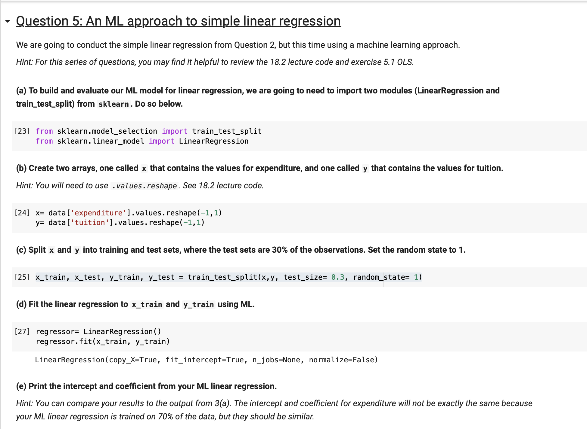
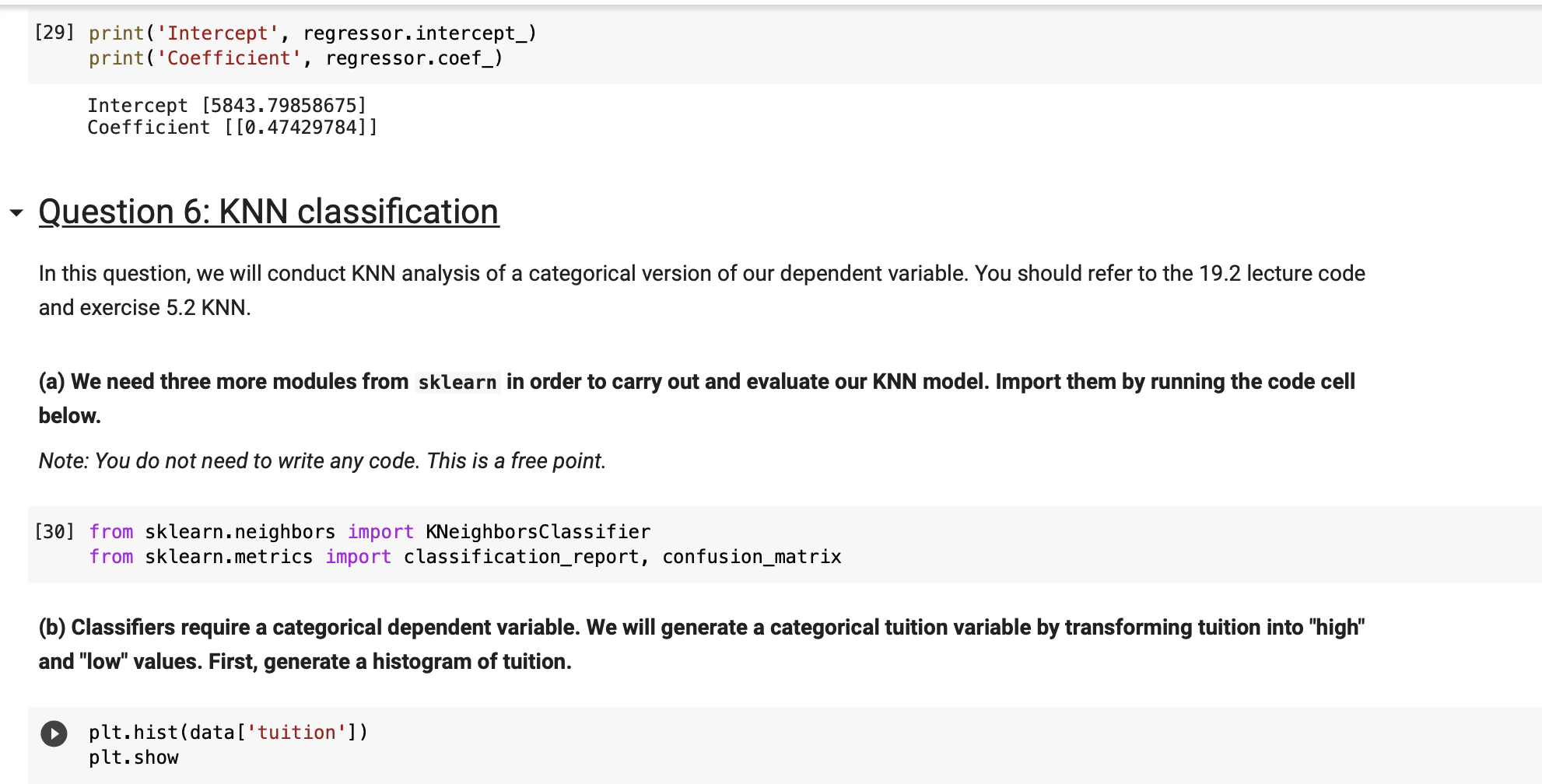
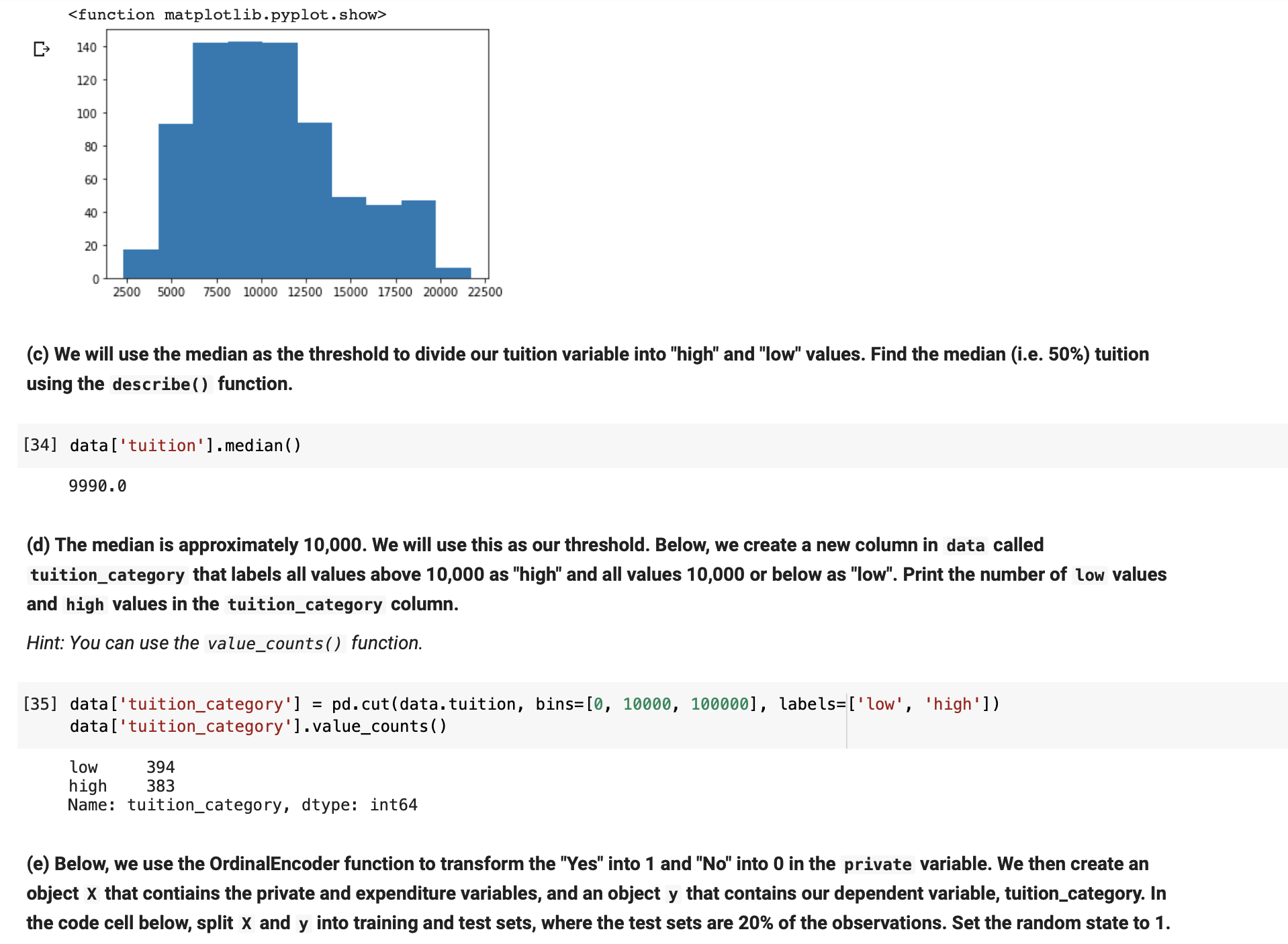
' Question 5: An ML approach to simple linear regression We are going to conduct the simple linear regression from Question 2, but this time using a machine learning approach. Hint: For this series of questions, you may find it helpful to review the 18.2 lecture code and exercise 5.1 OLS. (a) To build and evaluate our ML model for linear regression, we are going to need to import two modules (LinearRegression and train_test_split) from sktearn . Do so below. [23] from sklearn.model_selection import train_test_split from sklearn.linear_model import LinearRegression (b) Create two arrays, one called x that contains the values for expenditure, and one called y that contains the values for tuition. Hint: You will need to use . values. reshape. See 182 lecture code. [24] X: data['expenditure' ] .values. reshape(-1, 1) y= data['tuition'].va1ues. reshapel1,1l (c) Split x and y into training and test sets, where the test sets are 30% of the observations. Set the random state to 1 . [25] x_t rain, x_t_est_, y_t rain, y_test = train_test_split(x, y, test._size= a. 3, random_state= 1) (d) Fit the linear regression to x_t rain and y_t rain using ML. [27] regresser: LinearRegressionl) regressor.fit(x_train, y_train) LinearRegression(copy_X=True, fit_inter'cept=True, n_jobs=None, normalize=False) (e) Print the intercept and coefcient from your ML linear regression. Hint: You can compare your results to the output from 3(a). The intercept and coefficient for expenditure will not be exactly the same because your ML linear regression is trained on 70% of the data, but they should be similar. [29] print ( ' Intercept', regressor. intercept_) print ( 'Coefficient', regressor. coef_) Intercept [5843. 79858675] Coefficient [[0. 47429784]] . Question 6: KNN classification In this question, we will conduct KNN analysis of a categorical version of our dependent variable. You should refer to the 19.2 lecture code and exercise 5.2 KNN. (a) We need three more modules from sklearn in order to carry out and evaluate our KNN model. Import them by running the code cell below. Note: You do not need to write any code. This is a free point. [30] from sklearn. neighbors import KNeighborsClassifier from sklearn. metrics import classification_report, confusion_matrix (b) Classifiers require a categorical dependent variable. We will generate a categorical tuition variable by transforming tuition into "high" and "low" values. First, generate a histogram of tuition. plt. hist (data [' tuition' ] ) plt . 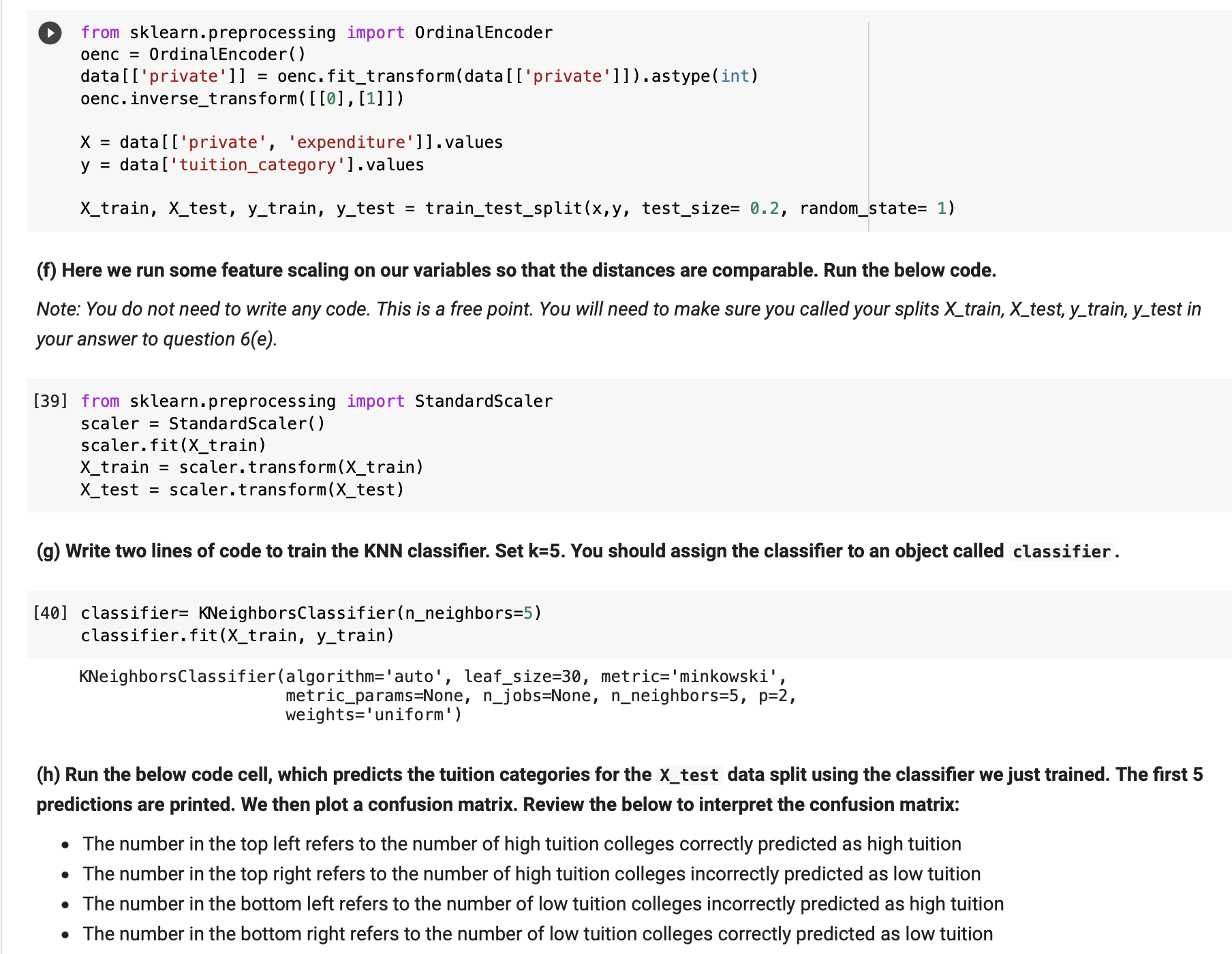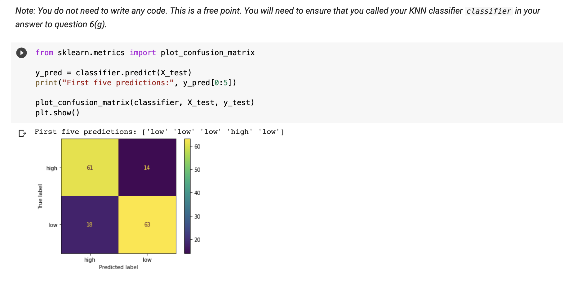show I} 140 120 100 8 8 8 8 O 2500 5000 1500 10000 12500 15000 17500 20000 22500 (c) We will use the median as the threshold to divide our tuition variable into "high" and "low'l values. Find the median (i.e. 50%) tuition using the describe() function. [34] datal'tuition'].medianl) 9990.0 (cl) The median is approximately 10,000. We will use this as our threshold. Below, we create a new column in data called tuition_category that labels all values above 10,000 as "high" and all values 10,000 or below as "low". Print the number of low values and high values in the tuition_category column. Hint: You can use the value_counts() function. [35] data['tuition_category'] = pd.cut(data.tuition, bins=[0, 10000, 100000], labels=['low', 'high']) data [ ' tuition_category '] .value_counts () low 394 high 383 Name: tuition_category, dtype: int64 (e) Below, we use the OrdinalEncoder function to transform the "Yes" into 1 and "No" into 0 in the private variable. We then create an object x that contiains the private and expenditure variables, and an object y that contains our dependent variable, tuition_category. In the code cell below, split x and y into training and test sets, where the test sets are 20% of the observations. Set the random state to 1 . D from sklearn. preprocessing import OrdinalEncoder oenc = OrdinalEncoder ( ) data [ [ 'private' ]] = oenc. fit_transform(data [ ['private' ]]) . astype(int) oenc. inverse_transform( [ [0] , [1] ] ) X = data [ ['private', 'expenditure' ]]. values y = data [' tuition_category' ] . values X_train, X_test, y_train, y_test = train_test_split(x,y, test_size= 0.2, random_state= 1) (f) Here we run some feature scaling on our variables so that the distances are comparable. Run the below code. Note: You do not need to write any code. This is a free point. You will need to make sure you called your splits X_train, X_test, y_train, y_test in your answer to question 6(e). [39] from sklearn. preprocessing import StandardScaler scaler = StandardScaler( ) scaler . fit (X_train) X_train = scaler. transform(X_train) X_test = scaler. transform(X_test) (g) Write two lines of code to train the KNN classifier. Set k=5. You should assign the classifier to an object called classifier. [40] classifier= KNeighborsClassifier(n_neighbors=5) classifier. fit(X_train, y_train) KNeighborsClassifier(algorithm='auto', leaf_size=30, metric='minkowski', metric_params=None, n_jobs=None, n_neighbors=5, p=2, weights=' uniform' ) (h) Run the below code cell, which predicts the tuition categories for the X_test data split using the classifier we just trained. The first 5 predictions are printed. We then plot a confusion matrix. Review the below to interpret the confusion matrix: . The number in the top left refers to the number of high tuition colleges correctly predicted as high tuition . The number in the top right refers to the number of high tuition colleges incorrectly predicted as low tuition . The number in the bottom left refers to the number of low tuition colleges incorrectly predicted as high tuition . The number in the bottom right refers to the number of low tuition colleges correctly predicted as low tuitionNote: You do not need to write any code. This is a free point. You will need to ensure that you called your KNN classifier classifier in your answer to question 6(g). from sklearn.metrics import plot_confusion_matrix y_pred = classifier. predict(X_test) print ("First five predictions:", y_pred [0:5]) plot_confusion_matrix(classifier, X_test, y_test) pit. show( ) First five predictions: ['low' 'low' 'low' 'high' 'low' ] 60 high 61 14 50 - 40 True label 30 low 18 63 20 high low Predicted label