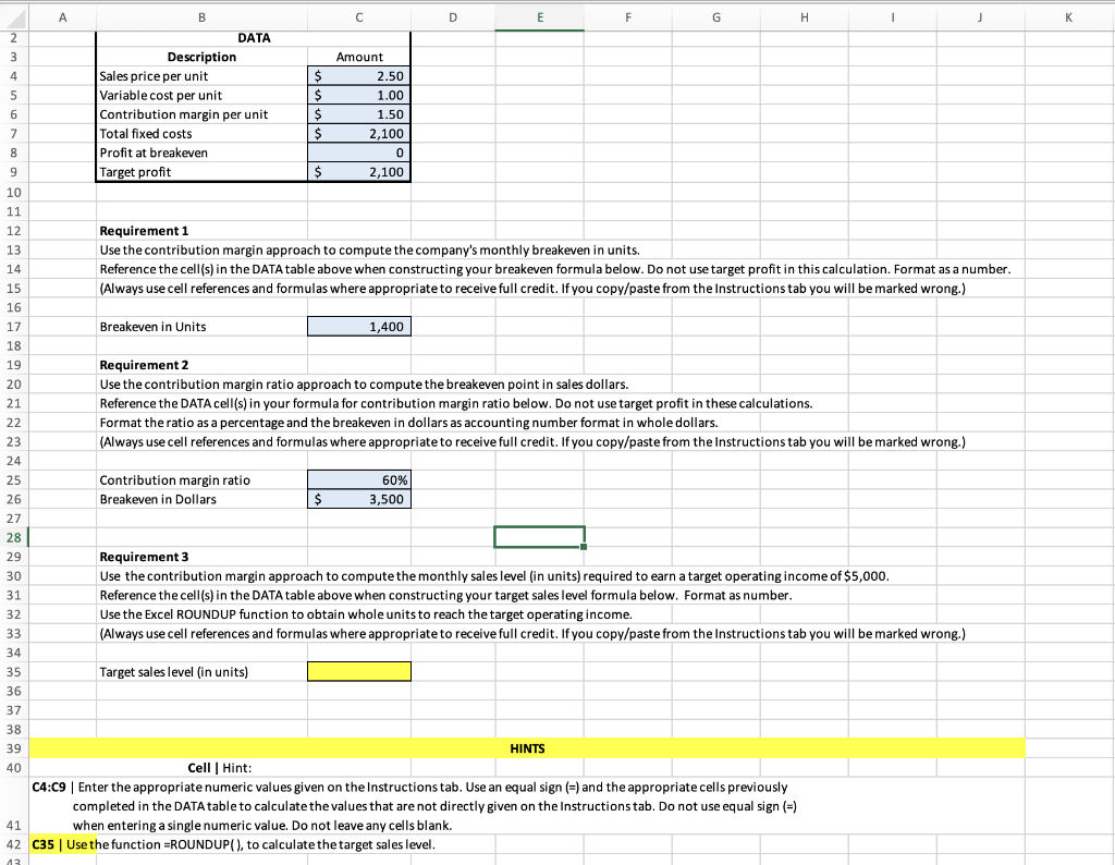
Hi! I need help with the last step. Please solve with the correct formula for excel, please.

A E F G H I J K DATA Sales price per unit $ 2.50 Variable cost per unit $ 1.00 Contribution margin per unit $ 1.50 Total fixed costs $ 2,100 Profit at breakeven 0 9 Target profit $ 2,100 10 11 12 Requirement 1 13 Use the contribution margin approach to compute the company's monthly breakeven in units. 14 Reference the cell(s) in the DATA table above when constructing your breakeven formula below. Do not use target profit in this calculation. Format as a number. (Always use cell references and formulas where appropriate to receive full credit. If you copy/paste from the Instructions tab you will be marked wrong.) 15 16 17 Breakeven in Units 1,400 18 19 Requirement 2 20 Use the contribution margin ratio approach to compute the breakeven point in sales dollars. 21 Reference the DATA cell(s) in your formula for contribution margin ratio below. Do not use target profit in these calculations. Format the ratio as a percentage and the breakeven in dollars as accounting number format in whole dollars. 22 23 (Always use cell references and formulas where appropriate to receive full credit. If you copy/paste from the Instructions tab you will be marked wrong.) 24 25 Contribution margin ratio 60% 26 Breakeven in Dollars $ 3,500 27 28 29 Requirement 3 30 Use the contribution margin approach to compute the monthly sales level (in units) required to earn a target operating income of $5,000. Reference the cell(s) in the DATA table above when constructing your target sales level formula below. Format as number. 31 32 Use the Excel ROUNDUP function to obtain whole units to reach the target operating income. 33 (Always use cell references and formulas where appropriate to receive full credit. If you copy/paste from the Instructions tab you will be marked wrong.) 34 35 Target sales level (in units) 36 37 38 39 HINTS 40 Cell | Hint: C4:C9 | Enter the appropriate numeric values given on the Instructions tab. Use an equal sign (=) and the appropriate cells previously completed in the DATA table to calculate the values that are not directly given on the Instructions tab. Do not use equal sign (=) when entering a single numeric value. Do not leave any cells blank. 41 42 C35 | Use the function =ROUNDUP(), to calculate the target sales level. 13 2 3 4 5 6 7 8 B Description Amount D