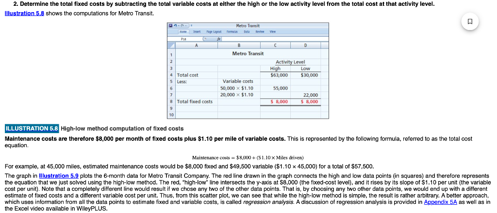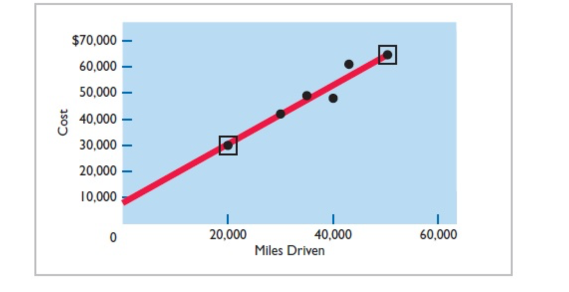
High-low method computation of fixed costs Maintenance costs are therefore $8,000 per month of fixed costs plus $1.10 per mile of variable costs. This is represented by the following formula, referred to as the total cost equation. Muintenance costs =$8,000+(S1.10 Miles driven ) For example, at 45,000 miles, estimated maintenance costs would be $8,000 fixed and $49,500 variable ($1.1045,000) for a total of $57,500. The graph in plots the 6-month data for Metro Transit Company. The red line drawn in the graph connects the high and low data points (in squares) and therefore represents the equation that we just solved using the high-low method. The red, "high-low" line intersects the y-axis at $8,000 (the fixed-cost level), and it rises by its slope of $1.10 per unit (the variable cost per unit). Note that a completely different line would result if we chose any two of the other data points. That is, by choosing any two other data points, we would end up with a different estimate of fixed costs and a different variable cost per unit. Thus, from this scatter plot, we can see that while the high-low method is simple, the result is rather arbitrary. A better approach, which uses information from all the data points to estimate fixed and variable costs, is called regression analysis. A discussion of regression analysis is provided in Appendix 5A as well as in the Excel video available in WileyPLUS. High-low method computation of fixed costs Maintenance costs are therefore $8,000 per month of fixed costs plus $1.10 per mile of variable costs. This is represented by the following formula, referred to as the total cost equation. Muintenance costs =$8,000+(S1.10 Miles driven ) For example, at 45,000 miles, estimated maintenance costs would be $8,000 fixed and $49,500 variable ($1.1045,000) for a total of $57,500. The graph in plots the 6-month data for Metro Transit Company. The red line drawn in the graph connects the high and low data points (in squares) and therefore represents the equation that we just solved using the high-low method. The red, "high-low" line intersects the y-axis at $8,000 (the fixed-cost level), and it rises by its slope of $1.10 per unit (the variable cost per unit). Note that a completely different line would result if we chose any two of the other data points. That is, by choosing any two other data points, we would end up with a different estimate of fixed costs and a different variable cost per unit. Thus, from this scatter plot, we can see that while the high-low method is simple, the result is rather arbitrary. A better approach, which uses information from all the data points to estimate fixed and variable costs, is called regression analysis. A discussion of regression analysis is provided in Appendix 5A as well as in the Excel video available in WileyPLUS