Question: HOMEWORK 7 1. A random sample of 700 cases or observations reveals 490 successes. Test whether the population proportion of successes is different from 0.65


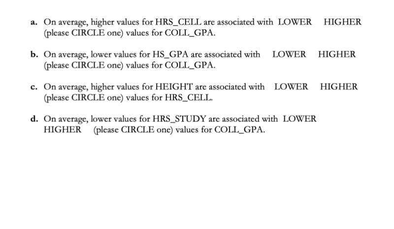
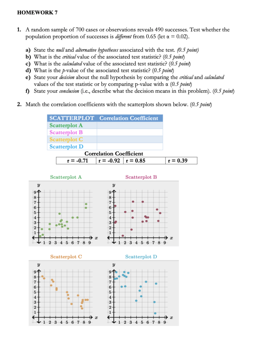
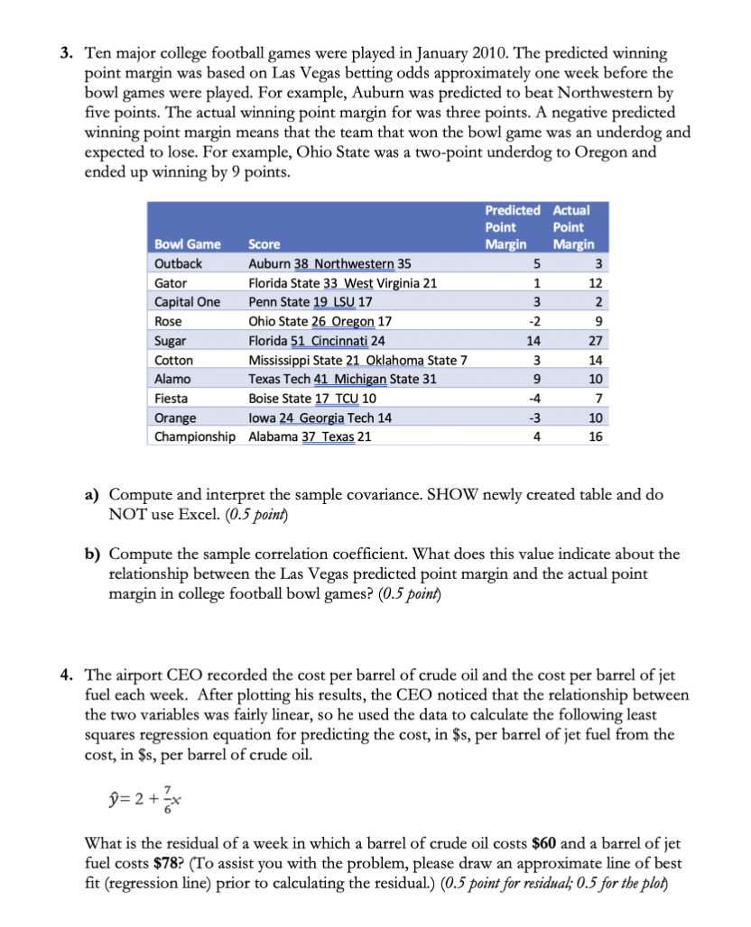
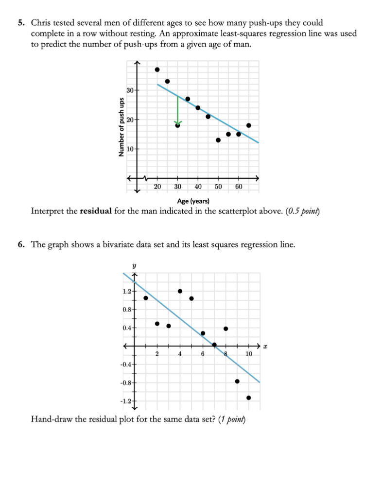
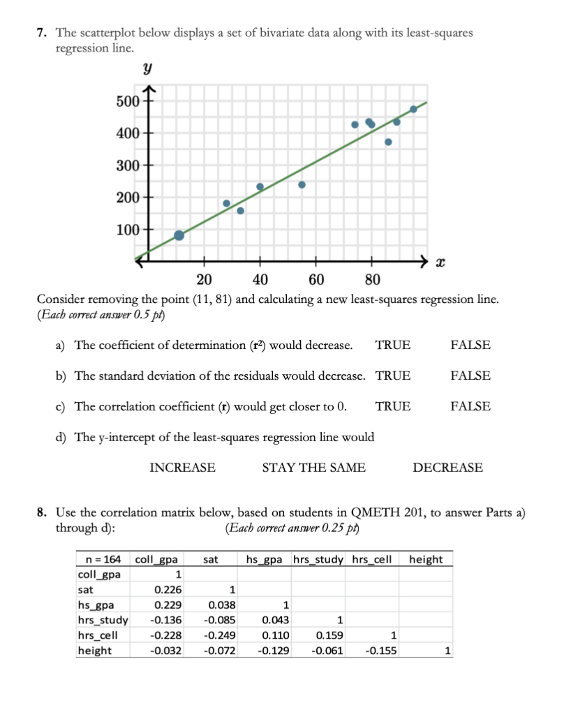

HOMEWORK 7 1. A random sample of 700 cases or observations reveals 490 successes. Test whether the population proportion of successes is different from 0.65 (let x = 0.02). a) State the null and alternative hypotheses associated with the test. (0.5 point) b) What is the critical value of the associated test statistic? (0.5 point) c) What is the calculated value of the associated test statistic? (0.5 point) d) What is the p-value of the associated test statistic? (0.5 point) e) State your decision about the null hypothesis by comparing the critical and calculated values of the test statistic or by comparing p-value with a (0.5 point) f) State your conclusion (i.e., describe what the decision means in this problem). (0.5 point) 2. Match the correlation coefficients with the scatterplots shown below. (0.5 point) SCATTERPLOT Correlation Coefficient Scatterplot A Scatterplot B Scatterplot C Scatterplot D Correlation Coefficient r = -0.71 r = -0.92 r = 0.85 r = 0.39 Scatterplot A Scatterplot B y y 94 8 - 7 - 6- 3- 7 8 9 Scatterplot C Scatterplot D y y 9 156789 1 2 4 567893. Ten major college football games were played in January 2010. The predicted winning point margin was based on Las Vegas betting odds approximately one week before the bowl games were played. For example, Auburn was predicted to beat Northwestern by five points. The actual winning point margin for was three points. A negative predicted winning point margin means that the team that won the bowl game was an underdog and expected to lose. For example, Ohio State was a two-point underdog to Oregon and ended up winning by 9 points. Predicted Actual Point Point Bowl Game Score Margin Margin Outback Auburn 38 Northwestern 35 5 3 Gator Florida State 33 West Virginia 21 12 W H Capital One Penn State 19 LSU 17 2 Rose Ohio State 26 Oregon 17 -2 9 Sugar Florida 51 Cincinnati 24 14 27 Cotton Mississippi State 21 Oklahoma State 7 3 14 Alamo Texas Tech 41 Michigan State 31 10 Fiesta Boise State 17 TCU 10 -4 7 Orange lowa 24 Georgia Tech 14 - 3 10 Championship Alabama 37 Texas 21 16 a) Compute and interpret the sample covariance. SHOW newly created table and do NOT use Excel. (0.5 point) b) Compute the sample correlation coefficient. What does this value indicate about the relationship between the Las Vegas predicted point margin and the actual point margin in college football bowl games? (0.5 point) 4. The airport CEO recorded the cost per barrel of crude oil and the cost per barrel of jet fuel each week. After plotting his results, the CEO noticed that the relationship between the two variables was fairly linear, so he used the data to calculate the following least squares regression equation for predicting the cost, in $s, per barrel of jet fuel from the cost, in $s, per barrel of crude oil. D= 2+-x What is the residual of a week in which a barrel of crude oil costs $60 and a barrel of jet fuel costs $78? (To assist you with the problem, please draw an approximate line of best fit (regression line) prior to calculating the residual.) (0.5 point for residual; 0.5 for the plot)5. Chris tested several men of different ages to see how many pushups they could complete in a row without testing. An approximate least-squares regression line was used to predict the number of push-ups from a given age of man. Me Mill's} Interpret the residual for the man indicated in the scattetplot above. (0.5% 6. The graph shows a biva'ate data set and its least squares regression line. I" Hand-draw the residual plot for the same data set? (I puma 7. The scatterplot below displays a set of bivariate data along with its least-squares regression line. y 500 7 400-+ 300 200-+ 100 20 40 60 80 Consider removing the point (11, 81) and calculating a new least-squares regression line. (Each correct answer 0.5 pt) a) The coefficient of determination (r2) would decrease. TRUE FALSE b) The standard deviation of the residuals would decrease. TRUE FALSE c) The correlation coefficient (r) would get closer to 0. TRUE FALSE d) The y-intercept of the least-squares regression line would INCREASE STAY THE SAME DECREASE 8. Use the correlation matrix below, based on students in QMETH 201, to answer Parts a) through d): (Each correct answer 0.25 pt) n = 164 coll_gpa sat hs_gpa hrs_study hrs_cell height coll_gpa sat 0.226 hs_gpa 0.229 0.038 1 hrs_study -0.136 -0.085 0.043 1 hrs_cell -0.228 -0.249 0.110 0.159 height -0.032 -0.072 -0.129 -0.061 -0.155 1a. On average, higher values for HRS_CELL are associated with LOWER HIGHER (please CIRCLE one) values for COLLGPA. b. On average, lower values for HS_GPA are associated with LOWER HIGHER (please CIRCLE one) values for COLL_GPA. c. On average, higher values for HEIGHT are associated with LOWER HIGHER (please CIRCLE one) values for HRS_CELL. d. On average, lower values for HRSjTUDY are associated with LOWER HIGHER {please CIRCLE one) values for COLL_GPA
Step by Step Solution
There are 3 Steps involved in it

Get step-by-step solutions from verified subject matter experts


