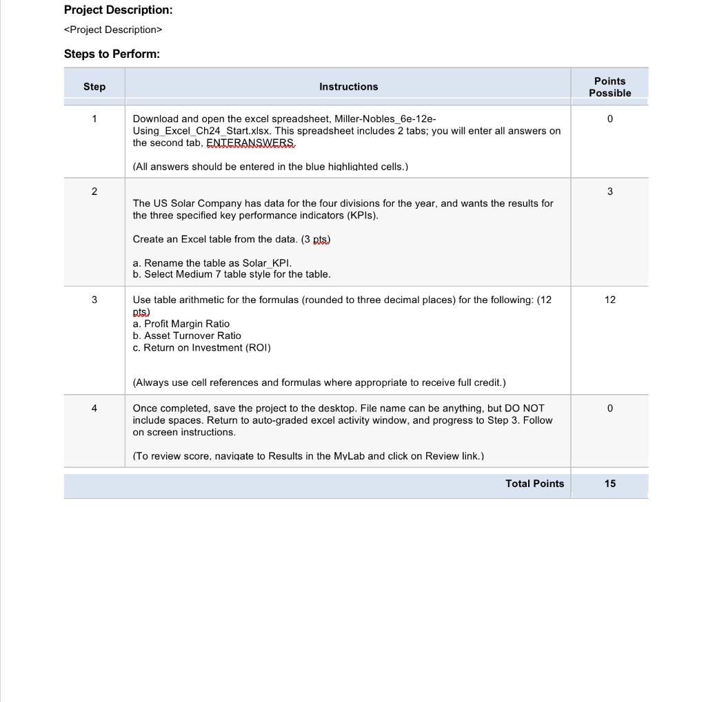
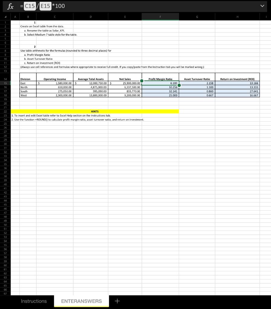
how do I enter the formula using ROUND() for profit margin / asset turnover ratio / roi

fx = C15/E15 * 100 B . D E H 1 Create an Excel table from the data a. Rename the table as Solar_KPI. b7 4 b. Select Medium 7 table style for the table. 5 6 7 10 11 12 13 2 Use table arithmetic for the formulas (rounded to three decimal places) for a. Profit Margin Ratio b. Asset Turnover Ratio c. Return on Investment (ROI) (Always use cell references and formulas where appropriate to receive full credit. If you copy/paste from the Instruction tab you will be marked wrong.) $ Division East North South West Operating Income 1,580,000.00 $ 650,000.00 275,050.00 2,300,000.00 Average Total Assets 12,000,750.00 $ 4,875,000.00 995,090.00 13,800,000.00 Net Sales 25,900,000.00 5,337,500.00 855,770.00 9,200,000.00 Profit Margin Ratio 6.100 10.256 32.141 25.000 Asset Turnover Ratio 2.158 1.300 0.860 0.667 Return on Investment (ROI) 13.166 13.333 27.641 16.667 HINTS 1. To insert and edit Excel table refer to Excel Help section on the instructions tab 2. Use the function =ROUND() to calculate profit margin ratio, asset turnover ratio, and return on investment 14 15 16. 17 18 19 20 21 22 23 24 25 26 27 28 29 30 31 32 33 34 35 36 37 38 39 40 41 42 43 44 45 46 47 48 49 50 51 52 53 54 55 56 57 58 59 60 61 62 63 64 65 66 67 Instructions ENTERANSWERS + Project Description: Steps to Perform: Step Instructions Points Possible 1 0 Download and open the excel spreadsheet, Miller-Nobles_6e-12e- Using Excel Ch24_Start.xlsx. This spreadsheet includes 2 tabs; you will enter all answers on the second tab, ENTERANSWERS (All answers should be entered in the blue highlighted cells.) 2 3 The US Solar Company has data for the four divisions for the year, and wants the results for the three specified key performance indicators (KPIs). Create an Excel table from the data. (3 pts) a. Rename the table as Solar_KPI. b. Select Medium 7 table style for the table. 3 12 Use table arithmetic for the formulas (rounded to three decimal places) for the following: (12 pts) a. Profit Margin Ratio b. Asset Turnover Ratio c. Return on Investment (ROI) (Always use cell references and formulas where appropriate to receive full credit.) 4 0 Once completed, save the project to the desktop. File name can be anything, but DO NOT include spaces. Return to auto-graded excel activity window, and progress to Step 3. Follow on screen instructions. (To review score, navigate to Results in the MyLab and click on Review link.) Total Points 15