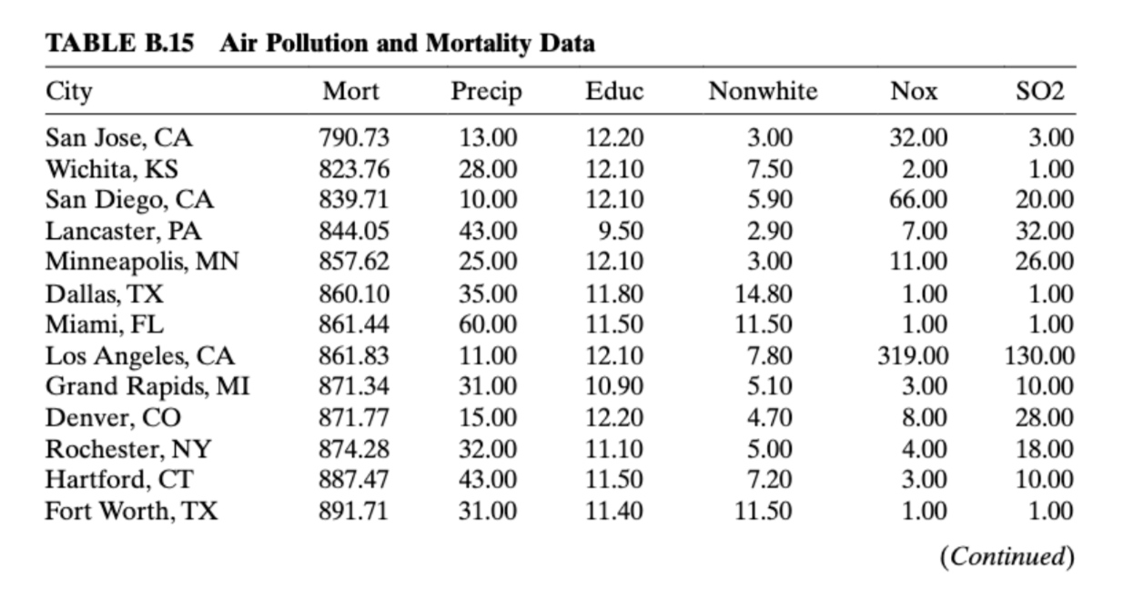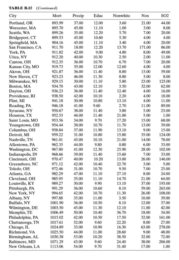


How does one reconcile multicolinearity in data once it is found? Chapter 9 mentions two popular choices: ridge regression (i.e., Kriging) and principle components regression. Consider the data found in Table B.15 detailing mortality and air pollution on a by city/demographic basis. Following Example 9.3, use principle-components regression in comparison with standard ordinary least squares. Highlight what relationships can be elucidated from the principle components.
Example 9.3 & Table B.15 data attached.
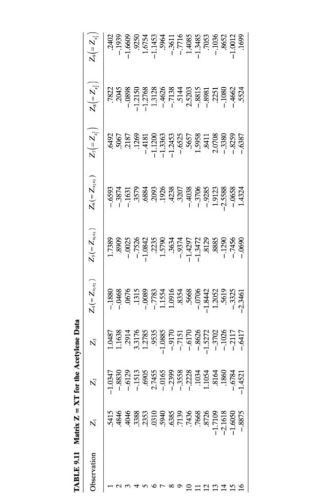
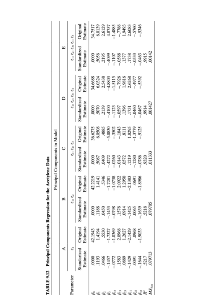
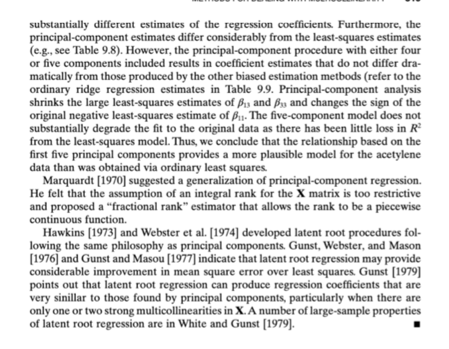
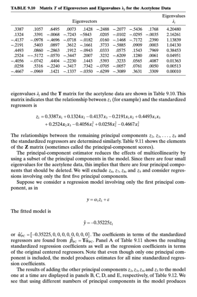
Example 9.3 Principal-Component Regression for the Acetylene Data We illustrate the use of principal-component regression for the acetylene data. We begin with the linear transformation Z = XT that transforms the original standard- ized regressors into an orthogonal set of variables (the principal components). TheTABLE 9.10 Matrix T of Eigenvectors and Eigenvalues a for the Acetylene Data Eigenvalues Eigenvectors .3387 .1057 .6495 .0073 .1428 -.2488 -2077 -5436 .1768 4.20480 .1324 .3391 -.0068 -.7243 -5843 0205 -.0102 -.0295 -.0035 2.16261 -.4137 -.0978 -4696 -.0718 -.0182 .0160 -.1468 -.7172 .2390 1.13839 -.2191 .5403 .0897 .3612 -.1661 3733 -.5885 .0909 .0003 1.04130 .4493 .0860 -.2863 .1912 -.0943 .0333 .0575 .1543 .7969 0.38453 .2524 -.5172 -.0570 -.3447 .2007 .3232 -.6209 .1280 .0061 0.04951 -.4056 -.0742 .4404 -.2230 .1443 .5393 .3233 .0565 .4087 0.01363 .0258 5316 -.2240 -3417 .7342 -.0705 -.0057 .0761 .0050 0.00513 -.4667 -.0969 .1421 -.1337 -.0350 -.6299 -.3089 .3631 .3309 0.00010 eigenvalues , and the T matrix for the acetylene data are shown in Table 9.10. This matrix indicates that the relationship between z, (for example) and the standardized regressors is 21 = 0.3387x, +0.1324x2 -0.4137x3 -0.2191x x2 +0.4493x1X'3 + 0.2524x2x3 -0.4056x3 +0.0258x3 -0.4667x} The relationships between the remaining principal components zz, Z, . .., z, and the standardized regressors are determined similarly. Table 9.11 shows the elements of the Z matrix (sometimes called the principal-component scores). The principal-component estimator reduces the effects of multicollinearity by using a subset of the principal components in the model. Since there are four small eigenvalues for the acetylene data, this implies that there are four principal compo- nents that should be deleted. We will exclude z6, Z7, Zs, and z, and consider regres- sions involving only the first five principal components. Suppose we consider a regression model involving only the first principal com- ponent, as in The fitted model is y =-0.35225z, or ape = [-0.35225, 0, 0, 0, 0, 0, 0, 0, 0]. The coefficients in terms of the standardized regressors are found from Bpc = Tape. Panel A of Table 9.11 shows the resulting standardized regression coefficients as well as the regression coefficients in terms of the original centered regressors. Note that even though only one principal com- ponent is included, the model produces estimates for all nine standardized regres- sion coefficients. The results of adding the other principal components zz, Z3, z., and zs to the model one at a time are displayed in panels B, C, D, and E, respectively, of Table 9.12. We see that using different numbers of principal components in the model produces\fTABLE 9.12 Principal Components Regression for the Acetylene Data Principal Components in Model U Parameter ZI. 21 ZI, Zz, 23 ZI, 21, 23, Z4 ZI, Zz, Z3, ZA, Zs Standarized Original Standardized Original Standardized Original Standardized Original Standardized Original Estimate Estimate Estimate Estimate Estimate Estimate Estimate Estimate Estimate Estimate .0000 42.1943 0000 42.2219 .0000 36.6275 .0000 34.6688 0000 34.7517 .1193 1.4194 .1188 1.4141 .5087 6.0508 .5070 6.0324 .5056 6.0139 .0466 .5530 .0450 .5346 .0409 .4885 .2139 2.5438 .2195 2.6129 -.1457 -1.7327 -.1453 -1.7281 -.4272 -5.0830 -.4100 -4.8803 -.4099 4.8757 -.0772 -1.0369 -.0798 -1.0738 -.0260 -.3502 -.1123 -1.5115 -.1107 -1.4885 .1583 2.0968 .1578 2.0922 -.0143 -.1843 -.0597 -.7926 -.0588 -.7788 .0889 1.2627 .0914 1.2950 .0572 .8111 .1396 1.9816 .1377 1.9493 -.1429 -2.1429 -.1425 -2.1383 .1219 1.8295 .1751 2.6268 .1738 2.6083 .0091 .0968 .0065 .0691 -.1280 -1.3779 -.0460 -.4977 -.0533 -.5760 -.1644 -1.9033 -.1639 -1.8986 -.0786 -.9125 -.0467 -.5392 -.0463 -.5346 .5217 .5218 .9320 .9914 .9915 MSRes .079713 .079705 .011333 .001427 .00142substantially different estimates of the regression coefficients. Furthermore, the principal-component estimates differ considerably from the least-squares estimates (e.g., see Table 9.8). However, the principal-component procedure with either four or five components included results in coefficient estimates that do not differ dra- matically from those produced by the other biased estimation metbods (refer to the ordinary ridge regression estimates in Table 9.9. Principal-component analysis shrinks the large least-squares estimates of Sis and By3 and changes the sign of the original negative least-squares estimate of 1. The five-component model does not substantially degrade the fit to the original data as there has been little loss in R? from the least-squares model. Thus, we conclude that the relationship based on the first five principal components provides a more plausible model for the acetylene data than was obtained via ordinary least squares. Marquardt [1970] suggested a generalization of principal-component regression. He felt that the assumption of an integral rank for the X matrix is too restrictive and proposed a "fractional rank" estimator that allows the rank to be a piecewise continuous function. Hawkins [1973] and Webster et al. [1974] developed latent root procedures fol- lowing the same philosophy as principal components. Gunst, Webster, and Mason [1976] and Gunst and Masou [1977] indicate that latent root regression may provide considerable improvement in mean square error over least squares. Gunst [1979] points out that latent root regression can produce regression coefficients that are very sinillar to those found by principal components, particularly when there are only one or two strong multicollinearities in X. A number of large-sample properties of latent root regression are in White and Gunst [1979].TABLE B.15 Air Pollution and Mortality Data City Mort Precip Educ Nonwhite Nox SO2 San Jose, CA 790.73 13.00 12.20 3.00 32.00 3.00 Wichita, KS 823.76 28.00 12.10 7.50 2.00 1.00 San Diego, CA 839.71 10.00 12.10 5.90 66.00 20.00 Lancaster, PA 844.05 43.00 9.50 2.90 7.00 32.00 Minneapolis, MN 857.62 25.00 12.10 3.00 11.00 26.00 Dallas, TX 860.10 35.00 11.80 14.80 1.00 1.00 Miami, FL 861.44 60.00 11.50 11.50 1.00 1.00 Los Angeles, CA 861.83 11.00 12.10 7.80 319.00 130.00 Grand Rapids, MI 871.34 31.00 10.90 5.10 3.00 10.00 Denver, CO 871.77 15.00 12.20 4.70 8.00 28.00 Rochester, NY 874.28 32.00 11.10 5.00 4.00 18.00 Hartford, CT 887.47 43.00 11.50 7.20 3.00 10.00 Fort Worth, TX 891.71 31.00 11.40 11.50 1.00 1.00 (Continued)


