I did not understand the article, Can you please briefly summarize the article.

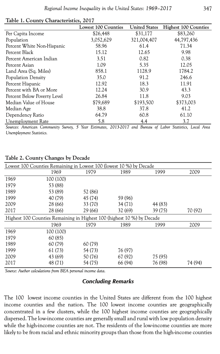
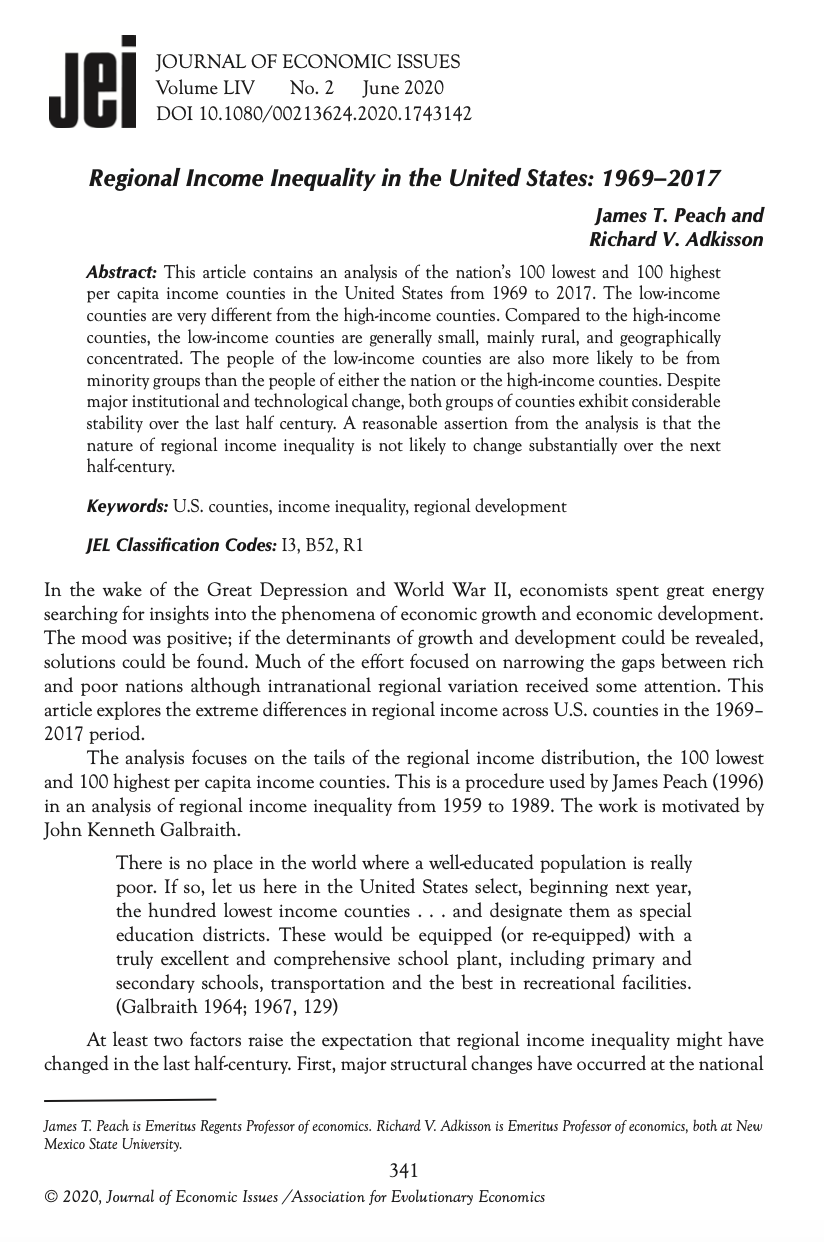
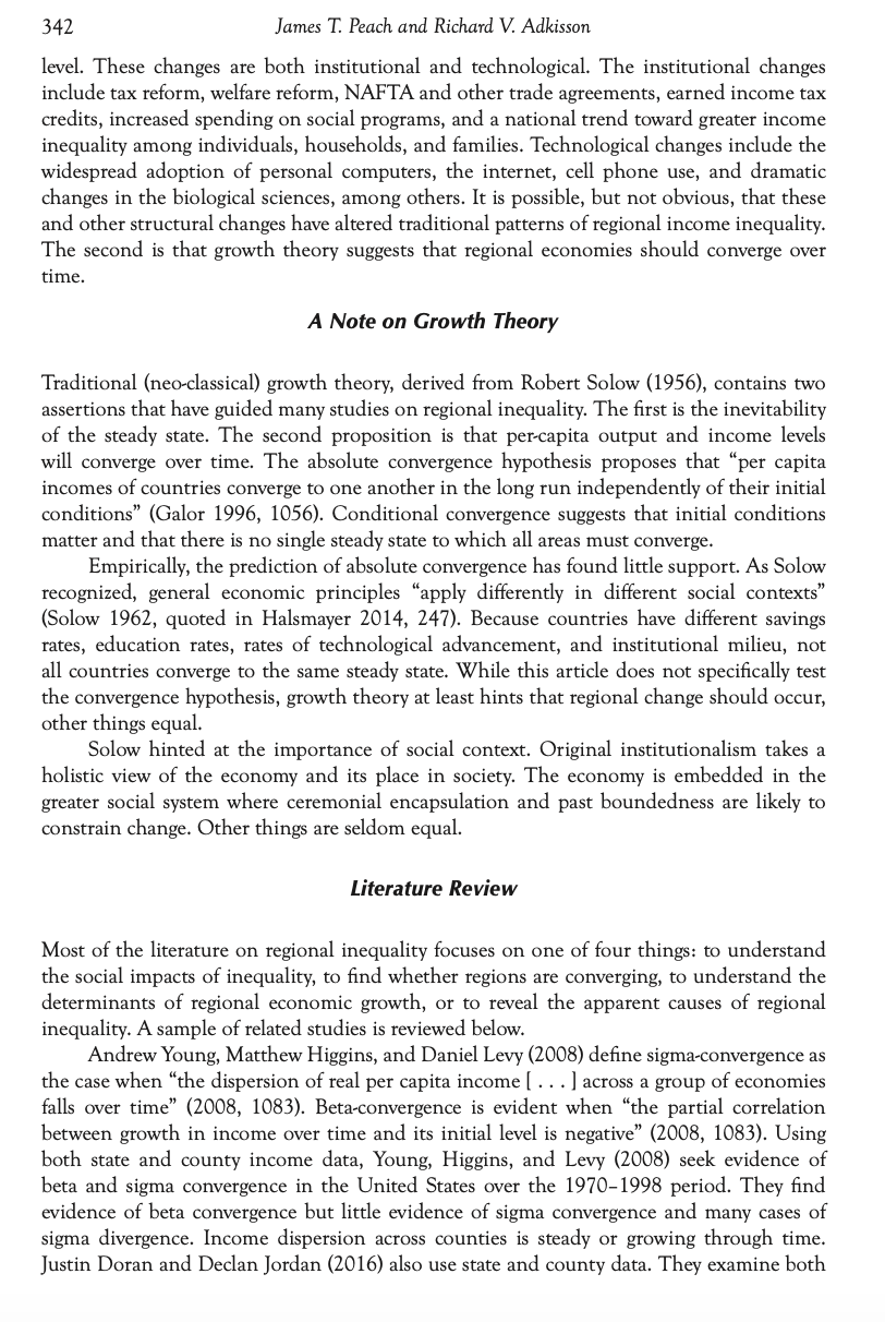
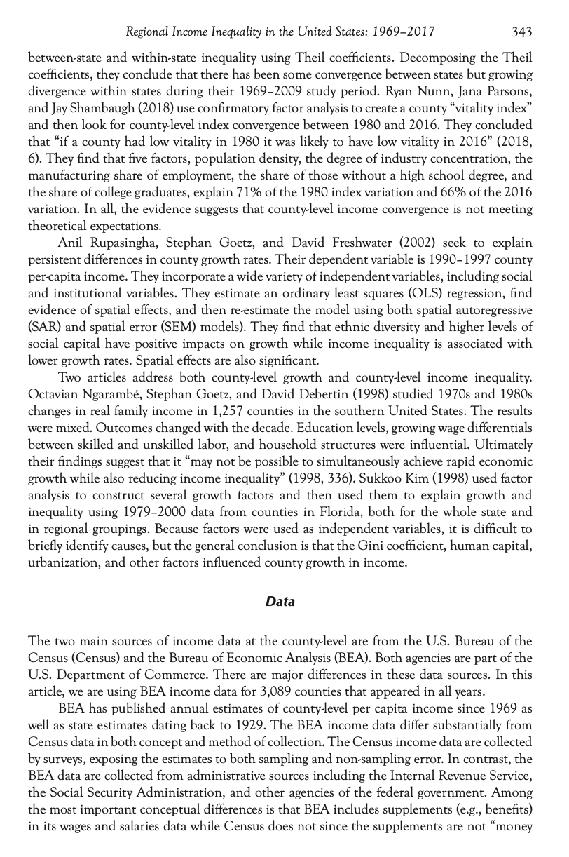
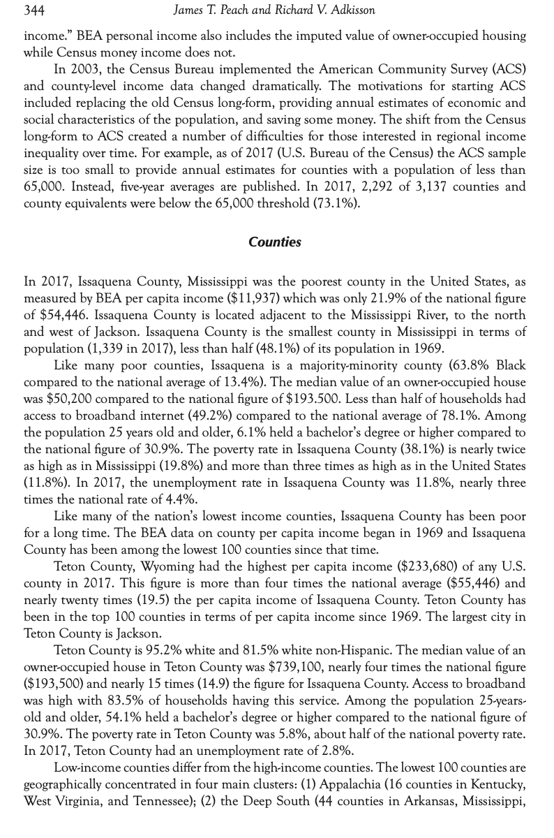
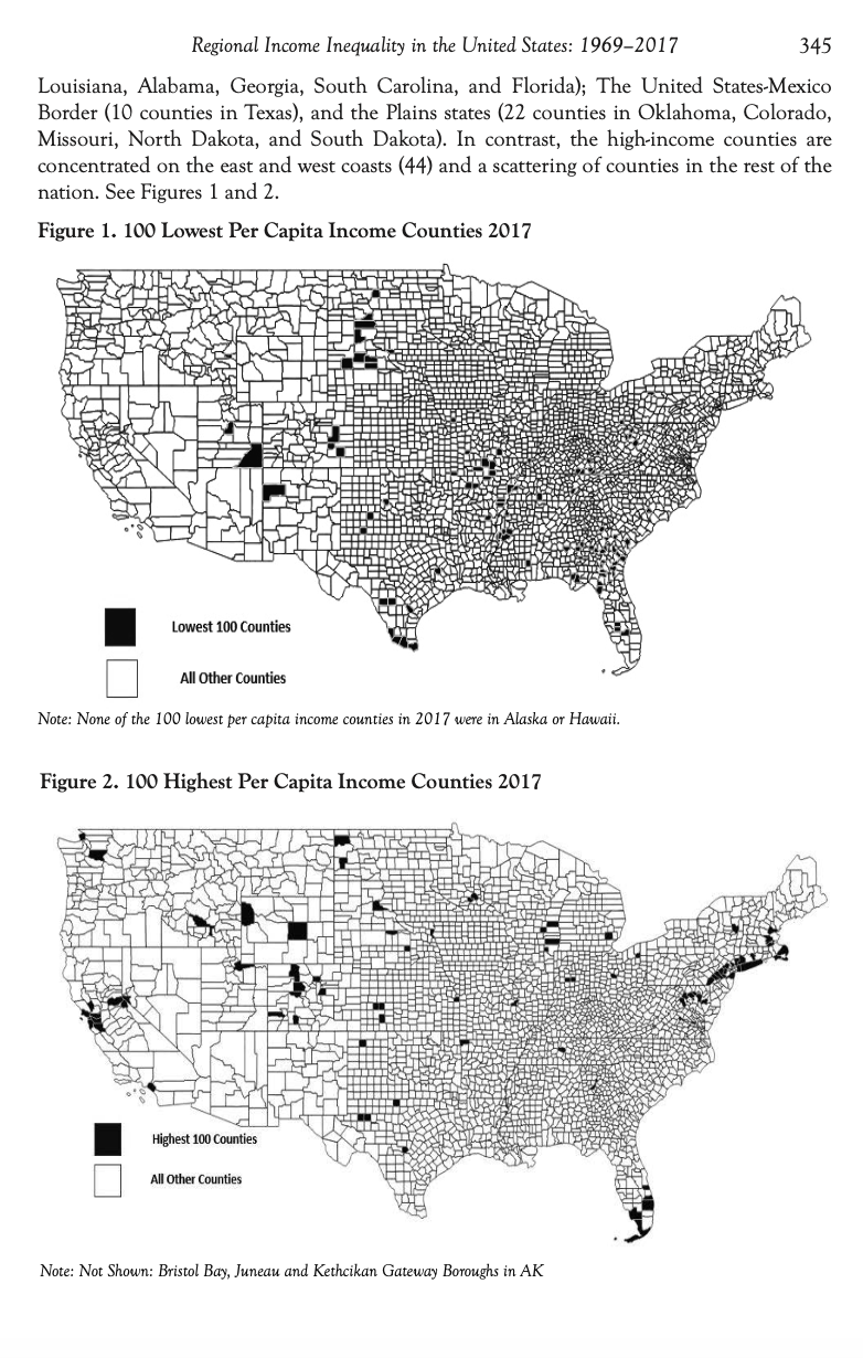
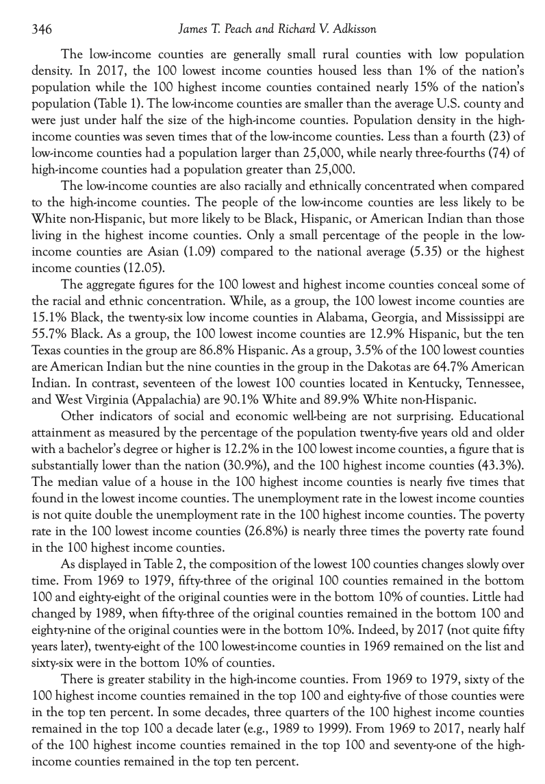
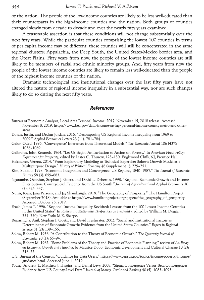
I JOURNAL OF ECONOMIC ISSUES Volume LIV No. 2 June 2020 DOI 10.1080/00213 624.2020. N43 142 Regional income Inequality in the United States: \"1969201 7 James T. Peach and Richard V. Adkisson Abstract: This article contains an analysis of the nation's 100 lowest and 100 highest per capita income counties in the United States from 1969 to 2017. The low-income counties are very different from the high-income counties. Compared to the high-income counties, the low-income counties are generally small, mainly rural, and geographically concentrated. The people of the lowdincome counties are also more likely to be from minority groups than the people of either the nation or the high-income counties. Despite major institutional and technological change, both groups of counties exhibit considerable stability over the last half century. A reasonable assertion from the analysis is that the nature of regional income inequality is not likely to change substantially over the next half-century. Keywords: U.S. counties, income inequality, regional development JEi. Classication Codes: [3, 352, R1 In the wake of the Great Depression and World War 11, economists spent great energy searching for insights into the phenomena of economic growth and economic development. The mood was positive; if the determinants of growth and development could be revealed, solutions could be found. Much of the effort focused on narrowing the gaps between rich and poor nations although intranational regional variation received some attention. This article explores the extreme differences in regional income across US. counties in the 1969 2017 period. The analysis focuses on the tails of the regional income distribution, the 100 lowest and 100 highest per capita income counties. This is a procedure used by James Peach (1996) in an analysis of regional income inequality from 1959 to 1989. The work is motivated by John Kenneth Galbraith. There is no place in the world where a well-educated population is really poor. If so, let us here in the United States select, beginning next year, the hundred lowest income counties . . . and designate them as special education districts. These would be equipped (or reequipped) with a truly excellent and comprehensive school plant, including primary and secondary schools, transportation and the best in recreational facilities. (Galbraith 1964; 1967. 129) At least two factors raise the expectation that regional income inequality might have changed in the last half-century. First, major structural changes have occurred at the national James T. Peach is Emerims Regen: meessor of economics. Richard V. Adkisson is Emeritus Prossor ofeoonomics. both at New Mexico State Unisem'ty. 341 2020, Journal of Economic Issues XAssociation for Evolutionary Econmnics 342 James I Peach and Ricl'mrd V. Adler'sson level These changes are both institutional and technological. The institutional changes include tax reform, welfare reform, NAFTA and other trade agreements, earned income tax credits, increased spending on social programs, and a national trend toward greater income inequality among individuals, households, and families. Technological changes include the widespread adoption of personal computers, the internet, cell phone use, and dramatic changes in the biological sciences, among others. It is possible, but not obvious, that these and other structural changes have altered traditional patterns of regional income inequality. The second is that growth theory suggests that regional economies should converge over time. A Note an Crowd: Theory Traditional (neoclassical) growth theory, derived from Robert Solow (1956), contains two assertions that have guided many studies on regional inequality. The rst is the inevitability of the steady state. The second proposition is that per-capita output and income levels will converge over time. The absolute convergence hypothesis proposes that \"per capita incomes of countries converge to one another in the long run independently of their initial conditions" (Galor 1996, 1056). Conditional convergence suggests that initial conditions matter and that there is no single steady state to which all areas must converge. Empirically, the prediction of absolute convergence has found little support. As Solow recognized, general economic principles \"apply differently in different social contexts" (Solow 1962, quoted in Halsmayer 2014, 247). Because countries have different savings rates, education rates, rates of technological advancement, and institutional milieu, not all countries converge to the same steady state. While this article does not specically test the convergence hypothesis, growth theory at least hints that regional change should occur, other things equal. Solow hinted at the importance of social context. Original institutionalism takes a holistic view of the economy and its place in society. The economy is embedded in the greater social system where ceremonial encapsulation and past boundedness are likely to constrain change. Other things are seldom equaL literature Review Most of the literature on regional inequality focuses on one of four things: to understand the social impacts of inequality, to nd whether regions are converging, to understand the determinants of regional economic growth, or to reveal the apparent causes of regional inequality. A sample of related studies is reviewed below. Andrew Young, Matthew Higgins, and Daniel Levy (2008) dene sigma-convergence as the case when \"the dispersion of real per capita income [ . . . ] across a group of economies falls over time" (2008, 1083). Beta-convergence is evident when \"the partial correlation between growth in income over time and its initial level is negative" (2008, 1083). Using both state and county income data, Young, Higgins, and Levy (2008) seek evidence of beta and sigma convergence in the United States over the 1970- 1998 period. They nd evidence of beta convergence but little evidence of sigma convergence and many cases of sigma divergence. Income dispersion across counties is steady or growing through time. Justin Doran and Declan Jordan (2016) also use state and county data. They examine both Regional income inequality in the United States: 1969201 7 343 between-state and within-state inequality using Theil coefficients. Decomposing the Theil coefcients, they conclude that there has been some convergence between states but growing divergence within states during their 1969-2009 study period. Ryan Nunn, Jana Parsons, and Jay Shambaugh (2018) use conrmatory factor analysis to create a county \"vitality index" and then look for county-level index convergence between 1980 and 2016. They concluded that \"if a county had low vitality in 1980 it was likely to have low vitality in 2016\" (2018, 6). They nd that ve factors, population density, the degree of industry concentration, the manufacturing share of employment, the share of those without a high school degree, and the share of college graduates, explain T196 of the 1980 index variation and 66% of the 2016 variation. In all, the evidence suggests that county-level income convergence is not meeting theoretical expectations. Anil Rupasingha, Stephan Goetz, and David Freshwater (2002) seek to explain persistent differences in county growth rates. Their dependent variable is 1990-1997 county per-capita income. They incorporate a wide variety of independent variables, including social and institutional variables. They estimate an ordinary least squares (OLS) regression, nd evidence of spatial effects, and then re-estimate the model using both spatial autoregressive {SAR) and spatial error (SEM) models). They nd that ethnic diversity and higher levels of social capital have positive impacts on growth while income inequality is associated with lower growth rates. Spatial effects are also signicant. Two articles address both county-level growth and county-level income inequality. Octavian Ngaramb, Stephan Goetz, and David Debertin (1998) studied 19705 and 1980s changes in real family income in 1,257 counties in the southern United States. The results were mixed. Outcomes changed with the decade. Education levels, growing wage differentials between skilled and unskilled labor, and household structures were influential. Ultimately their ndings suggest that it \"may not be possible to simultaneously achieve rapid economic growth while also reducing income inequality\" {1998, 336). Sukkoo Kim (1998) used factor analysis to construct several growth factors and then used them to explain growth and inequality using 1979-2000 data from counties in Florida, both for the whole state and in regional groupings. Because factors were used as independent variables, it is difcult to briey identify causes, but the general conclusion is that the Gini coefcient, human capital, urbanization, and other factors inuenced county growth in income. Da ta The two main sources of income data at the county-level are from the US. Bureau of the Census (Census) and the Bureau of Economic Analysis (BEA). Both agencies are part of the US. Department of Commerce. There are major differences in these data sources. In this article, we are using BEA income data for 3,039 counties that appeared in all years. BEA has published annual estimates of county-level per capita income since 1969 as well as state estimates dating back to 1929. The BEA income data differ substantially from Census data in both concept and method of collection. The Census income data are collected by surveys, exposing the estimates to both sampling and non-sampling error. In contrast, the BEA data are collected from administrative sources including the Internal Revenue Service, the Social Security Administration, and other agencies of the federal government. Among the most important conceptual differences is that BEA includes supplements (e.g., benets) in its wages and salaries data while Census does not since the supplements are not \"money 344 James T. Peach and Richard V. Adkisson income." BEA personal income also includes the imputed value of owner-occupied housing while Census money income does not. In 2003, the Census Bureau implemented the American Community Survey (ACS) and county-level income data changed dramatically. The motivations for starting ACS included replacing the old Census long-form, providing annual estimates of economic and social characteristics of the population, and saving some money. The shift from the Census long-form to ACS created a number of difficulties for those interested in regional income inequality over time. For example, as of 2017 (U.S. Bureau of the Census) the ACS sample size is too small to provide annual estimates for counties with a population of less than 65,000. Instead, five-year averages are published. In 2017, 2,292 of 3,137 counties and county equivalents were below the 65,000 threshold (73.1%). Counties In 2017, Issaquena County, Mississippi was the poorest county in the United States, as measured by BEA per capita income ($11,937) which was only 21.9% of the national figure of $54,446. Issaquena County is located adjacent to the Mississippi River, to the north and west of Jackson. Issaquena County is the smallest county in Mississippi in terms of population (1,339 in 2017), less than half (48.1%) of its population in 1969. Like many poor counties, Issaquena is a majority-minority county (63.8% Black compared to the national average of 13.4%). The median value of an owner-occupied house was $50,200 compared to the national figure of $193.500. Less than half of households had access to broadband internet (49.2%) compared to the national average of 78.1%. Among the population 25 years old and older, 6.1% held a bachelor's degree or higher compared to the national figure of 30.9%. The poverty rate in Issaquena County (38.1%) is nearly twice as high as in Mississippi (19.8%) and more than three times as high as in the United States (11.8%). In 2017, the unemployment rate in Issaquena County was 11.8%, nearly three times the national rate of 4.4%. Like many of the nation's lowest income counties, Issaquena County has been poor for a long time. The BEA data on county per capita income began in 1969 and Issaquena County has been among the lowest 100 counties since that time. Teton County, Wyoming had the highest per capita income ($233,680) of any U.S. county in 2017. This figure is more than four times the national average ($55,446) and nearly twenty times (19.5) the per capita income of Issaquena County. Teton County has been in the top 100 counties in terms of per capita income since 1969. The largest city in Teton County is Jackson. Teton County is 95.2% white and 81.5% white non-Hispanic. The median value of an owner-occupied house in Teton County was $739,100, nearly four times the national figure ($193,500) and nearly 15 times (14.9) the figure for Issaquena County. Access to broadband was high with 83.5% of households having this service. Among the population 25-years- old and older, 54.1% held a bachelor's degree or higher compared to the national figure of 30.9%. The poverty rate in Teton County was 5.8%, about half of the national poverty rate. In 2017, Teton County had an unemployment rate of 2.8%. Low-income counties differ from the high-income counties. The lowest 100 counties are geographically concentrated in four main clusters: (1) Appalachia (16 counties in Kentucky, West Virginia, and Tennessee); (2) the Deep South (44 counties in Arkansas, Mississippi,Regional Income Inequality in the United States: 1969-2017 345 Louisiana, Alabama, Georgia, South Carolina, and Florida); The United States-Mexico Border (10 counties in Texas), and the Plains states (22 counties in Oklahoma, Colorado, Missouri, North Dakota, and South Dakota). In contrast, the high-income counties are concentrated on the east and west coasts (44) and a scattering of counties in the rest of the nation. See Figures 1 and 2. Figure 1. 100 Lowest Per Capita Income Counties 2017 Lowest 100 Counties All Other Counties Note: None of the 100 lowest per capita income counties in 2017 were in Alaska or Hawaii. Figure 2. 100 Highest Per Capita Income Counties 2017 Highest 100 Counties All Other Counties Note: Not Shown: Bristol Bay, Juneau and Ketheikan Gateway Boroughs in AK346 James T: Peach and Richard V. Adkisson. The low-income counties are generally small rural counties with low population density. In 201?, the 100 lowest income counties housed less than 1% of the nation's population while the 100 highest income counties contained nearly 15% of the nation's population (Table 1). The low-income counties are smaller than the average U. S. county and were just under half the size of the high-income counties. Population density in the high- income counties was seven times that of the low-income counties. Less than a fourth (23) of low-income counties had a population larger than 25,000, while nearly three-fourths (74) of high-income counties had a population greater than 25,000. The low-income counties are also racially and ethnically concentrated when compared to the high-income counties. The people of the low-income counties are less likely to be White non-Hispanic, but more likely to be Black, Hispanic, or American Indian than those living in the highest income counties. Only a small percentage of the people in the low- income counties are Asian (1.09) compared to the national average (5.35) or the highest income counties (12.05). The aggregate gures for the 100 lowest and highest income counties conceal some of the racial and ethnic concentration. While, as a group, the 100 lowest income counties are 15.1% Black, the twenty-six low income counties in Alabama, Georgia, and Mississippi are 55.7% Black. As a group, the 100 lowest income counties are 12.9% Hispanic, but the ten Texas counties in the group are 86.3% Hispanic. As a group, 3.5% of the 100 lowest counties are American Indian but the nine counties in the group in the Dakotas are 64.7% American Indian. In contrast, seventeen of the lowest 100 counties located in Kentucky, Tennessee, and West Virginia (Appalachia) are 90.1% White and 89.9% White nonrHispanic. Other indicators of social and economic well-being are not surprising. Educational attainment as measured by the percentage of the population twenty-ve years old and older with a bachelor's degree or higher is 12.2% in the 100 lowest income counties, a gure that is substantially lower than the nation (30.9%), and the 100 highest income counties (43.3%). The median value of a house in the 100 highest income counties is nearly ve times that found in the lowest income counties. The unemployment rate in the lowest income counties is not quite double the unemployment rate in the 100 highest income counties. The poverty rate in the 100 lowest income counties (26.3%) is nearly three times the poverty rate found in the 100 highest income counties. As displayed in Table 2, the composition of the lowest 100 counties changes slowly over time. From 1969 to 1979, ftyrthree of the original 100 counties remained in the bottom 100 and eighty-eight of the original counties were in the bottom 10% of counties. Little had changed by 1939, when fty-three of the original counties remained in the bottom 100 and eightyrnine of the original counties were in the bottom 10%. Indeed, by 201? (not quite fty years later), twenty-eight of the 100 lowest-income counties in 1969 remained on the list and sixtyrsix were in the bottom 10% of counties. There is greater stability in the high-income counties. From 1969 to 1979, sixty of the 100 highest income counties remained in the top 100 and eighty-ve of those counties were in the top ten percent. In some decades, three quarters of the 100 highest income counties remained in the top 100 a decade later (eg, 1989 to 1999). From 1969 to 2012, nearly half of the 100 highest income counties remained in the top 100 and seventy-one of the high- income counties remained in the top ten percent. Regional income inequality in the United States: 1969201 7 347 Table l. Coun Characteristics, 2017 lamest 100 Counties United States H' est 100 Counties Per Capita Income $26,443 $31,177 $83,260 Population 3,052,629 321,004,407 44,7 97,436 Percent White Non-Hispanic 53.96 61.4 7 1.34 Percent Black 15.12 12.65 9.98 Percent American Indian 3.5 1 0.32 0.38 Percent Asian 1.09 5.35 12.05 LandArealSq. Miles} 353.1 1128.9 1734.2 Population Density 35.0 91.2 246.6 Percent Hispanic 12.92 18.3 1 1.91 Percent with BA or More 12.24 30.9 43.3 Percent Below Poverty Level 26.34 11.3 9.03 Median Value of House $79,639 $193,500 $373,003 Median Age 38.8 37.3 41.2 Dependency Ratio 64.79 60.3 61.10 Unemployment Rate 5.3 4.4 3.7 Sources: American Community Survey, 5 Year Estimates, 20132017 and Bureau of Labor Statistics, local Area Unemployment Statistics. Table 2. County Changes by Decade Lowest 100 Counties Remaining in Lowest 100 (lowest 10 96} by Decade 1969 1979 1989 1999 2009 1969 100 (100} 1979 53 {88} 1989 53 {89} 52 {86} 1999 40 {79) 45 {74) 59 {96) 2009 23 {66} 33 {70} 34 {71} 44 {83} 2017 23 (66} 29 (66} 32 (69} 39 (75} 70 (92) Highest 100 Counties Remaining in Highest 100 (highest 10 '36) by Decade 1969 1979 1989 1999 2009 1969 100 {100) 1979 60 (851 1989 60 {79} 60 {79} 1999 61 {73) 54 {73) 76 {97) 2009 43 {69) 50 {76) 67 {92) 75 {95) 201? 48 a1) 54 W5) 66 {94) 76 {98) 74 {94) Source: Author calculations Jfrom BEA personal income data. Concluding Remarks The 100 lowest income counties in the United States are different from the 100 highest income counties and the nation. The 100 lowest income counties are geographically concentrated in a few clusters, while the 100 highest income counties are geographically dispersed. The low-income counties are generally small and rural with low population density while the high-income counties are not. The residents of the low-income counties are more likely to be from racial and ethnic minority groups than those from the high-income counties 348 James T. Peach and Richard V. Adkisson or the nation. The people of the low-income counties are likely to be less well-educated than their counterparts in the high-income counties and the nation. Both groups of counties changed slowly from decade to decade and over the nearly fifty years examined. A reasonable assertion is that these conditions will not change substantially over the next fifty years. While the particular counties comprising the lowest 100 counties in terms of per capita income may be different, these counties will still be concentrated in the same regional clusters: Appalachia, the Deep South, the United States-Mexico border area, and the Great Plains. Fifty years from now, the people of the lowest income counties are still likely to be members of racial and ethnic minority groups. And, fifty years from now the people of the lowest income counties are likely to remain less well-educated than the people of the highest income counties or the nation. Dramatic technological and institutional changes over the last fifty years have not altered the nature of regional income inequality in a substantial way, nor are such changes likely to do so during the next fifty years. References Bureau of Economic Analysis, Local Area Personal Income. 2017, November 15, 2018 release. Accessed November 8, 2019. https://www.bea.gov/data/income-saving/personal-income-county-metro-and-other- areas Doran, Justin, and Declan Jordan. 2016. "Decomposing US Regional Income Inequality from 1969 to 2009." Applied Economics Letters 23 (11): 781-784. Galor, Oded. 1996. "Convergence? Inferences from Theoretical Models." The Economic Journal 106 (437): 1056-1069. Galbraith, John Kenneth. 1964. "Let Us Begin: An Invitation to Action on Poverty." In American Fiscal Policy: Experiment for Prosperity, edited by Lester C. Thurow, 123-130. Englewood Cliffs, NJ; Prentice Hall. Halsmayer, Verena. 2014. "From Exploratory Modeling to Technical Expertise: Solow's Growth Model as a Multipurpose Design." History of Political Economy 46 (supplement 1): 229-251. Kim, Sukkoo. 1998. "Economic Integration and Convergence: US Regions, 1840-1987." The Journal of Economic History 58 (3): 659-683. Ngarambe, Octavian, Stephan J. Goetz, and David L. Debertin. 1998. "Regional Economic Growth and Income Distribution: County-Level Evidence from the US South." Journal of Agricultural and Applied Economics 30 2): 325-337. Nunn, Ryan, Jana Parsons, and Jay Shambaugh. 2018. "The Geography of Prosperity." The Hamilton Project September 2018). Available at https://www.hamiltonproject.org/papers/the_geography_of_prosperity. Accessed October 28, 2019. Peach, James T. 1996. "Regional Income Inequality Revisited: Lessons from the 100 Lowest Income Counties in the United States" In Radical Institutionalist Perspectives on Inequality, edited by William M. Dugger, 237-250). New York: M.E. Sharpe. Rupasingha, Anil, Stephan J. Goetz, and David Freshwater. 2002. "Social and Institutional Factors as Determinants of Economic Growth: Evidence from the United States Counties." Papers in Regional Science 81 (2): 139-155. Solow, Robert M. 1956. "A Contribution to the Theory of Economic Growth." The Quarterly Journal of Economics 70 (1): 65-94. Solow, Robert M. 1962. "Some Problems of the Theory and Practice of Economic Planning," review of An Essay on Economic Growth and Planning, by Maurice Dobb. Economic Development and Cultural Change 10 (2): 216-22. U.S. Bureau of the Census. "Guidance for Data Users." https://www.census.gov/topics/income-poverty/income/ guidance.html. Accessed June 4, 2019. Young, Andrew T., Matthew J. Higgins, and Daniel Levy. 2008. "Sigma Convergence Versus Beta Convergence: Evidence from US County-Level Data." Journal of Money, Credit and Banking 40 (5): 1083-1093