I have all the named ranges and data validations done already. EDIT: If possible could you tell me what equations to enter and where.

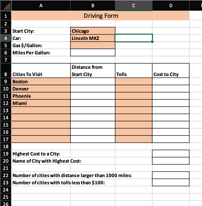
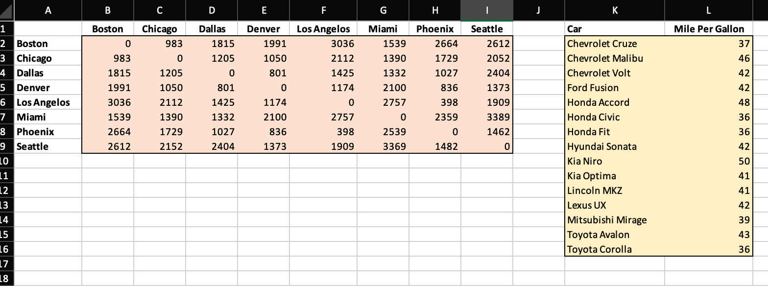
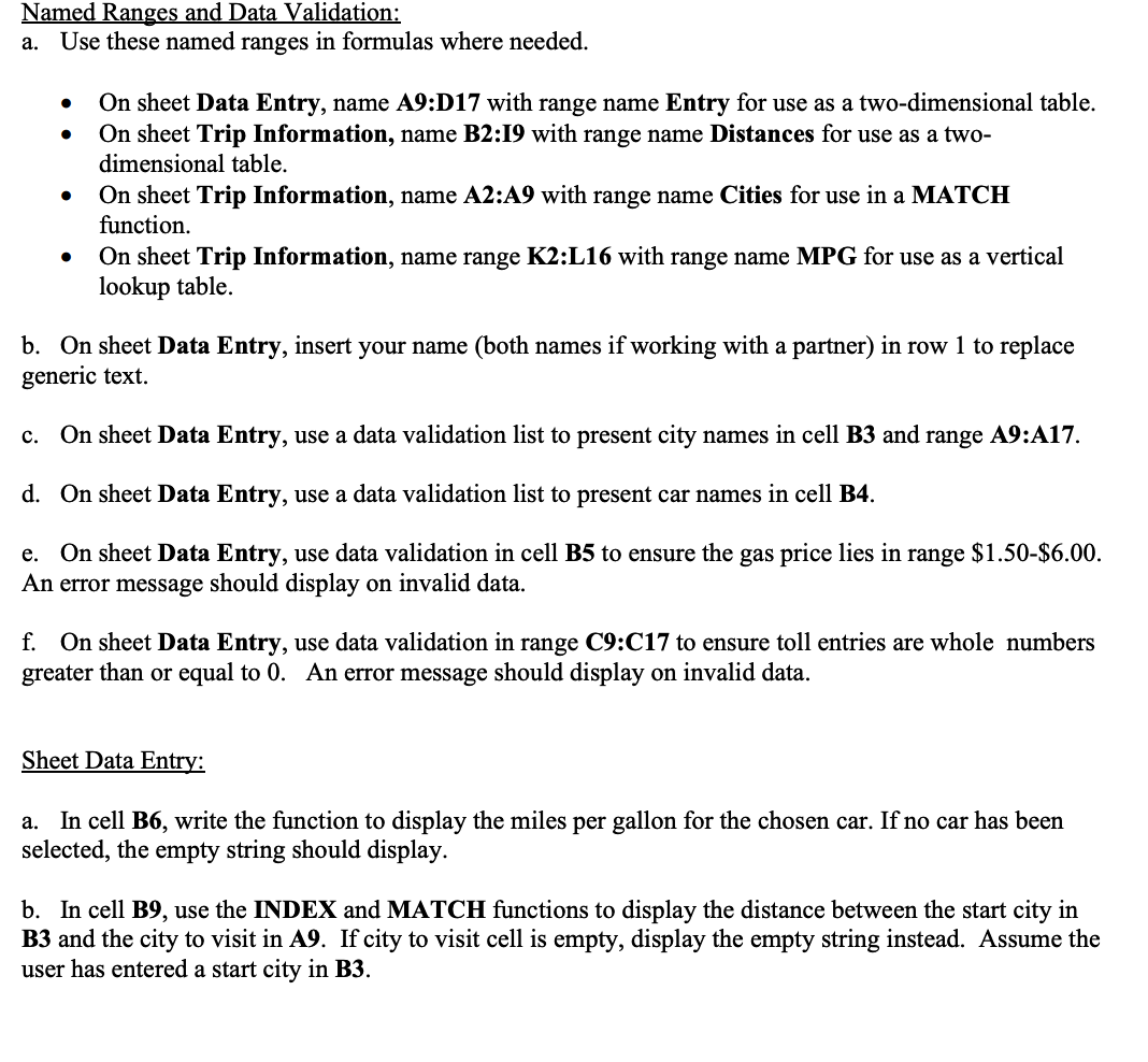
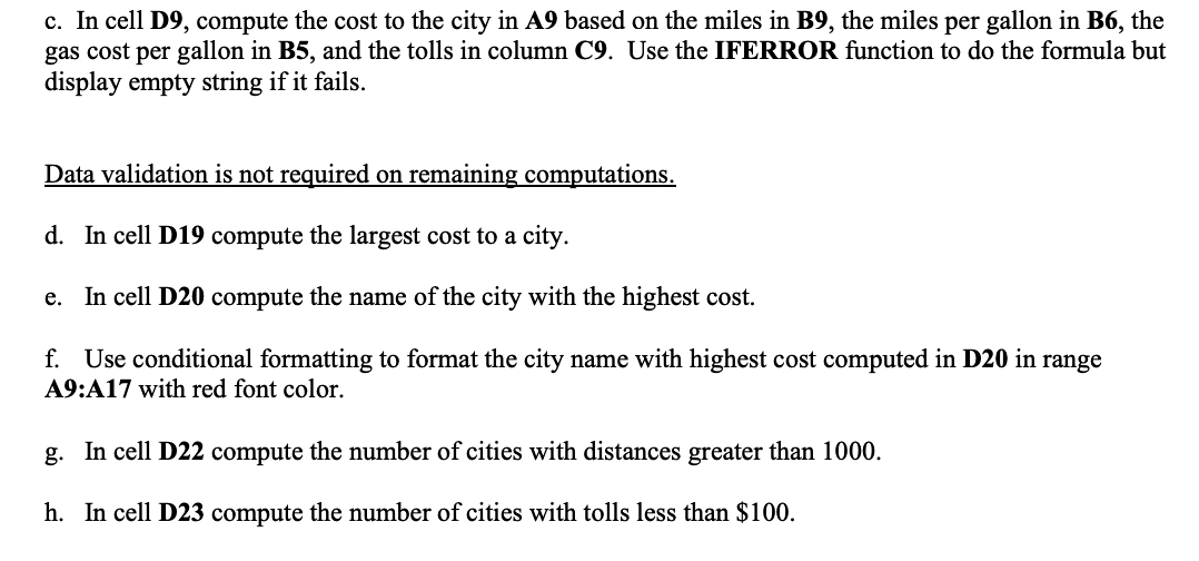
B Driving Form Chicago Lincoln MKZ 3 Start City: 4 Car: Gas $/Gallon: 6 Miles Per Gallon: Distance from Start City Tolls Cost to City 8 Cities To Visit 9 Boston 10 Denver 11 Phoenix 12 Miami 13 14 15 17 18 19 Highest Cost to a City: 20 Name of City with Highest Cost: 21 22 Number of cities with distance larger than 1000 miles: 23 Number of cities with tolls less than $100: 24 25 26 . Mile Per Gallon Chicago 983 o 2 Boston 3 Chicago 4 Dallas 5 Denver 6 Los Angelos 7 Miami 8 Phoenix 9 Seattle Boston 0 983 1815 1991 3036 1539 2664 2612 1205 1050 2112 1390 1729 2152 Dallas 1815 1205 0 801 1425 1332 1027 2404 Denver 1991 1050 801 0 1174 2100 836 1373 Los AngelosMiami 3036 1539 2112 1390 1425 1332 1174 2100 0 2757 2757 398 2539 1909 3369 Phoenix 2664 1729 1027 836 398 2359 Seattle 2612 2052 2404 1373 1909 3389 1462 0 Car Chevrolet Cruze Chevrolet Malibu Chevrolet Volt Ford Fusion Honda Accord Honda Civic Honda Fit Hyundai Sonata Kia Niro Kia Optima Lincoln MKZ Lexus UX Mitsubishi Mirage Toyota Avalon Toyota Corolla 1482 10 Named Ranges and Data Validation: a. Use these named ranges in formulas where needed. On sheet Data Entry, name A9:D17 with range name Entry for use as a two-dimensional table. On sheet Trip Information, name B2:19 with range name Distances for use as a two- dimensional table. On sheet Trip Information, name A2:A9 with range name Cities for use in a MATCH function. On sheet Trip Information, name range K2:L16 with range name MPG for use as a vertical lookup table. b. On sheet Data Entry, insert your name (both names if working with a partner) in row 1 to replace generic text. c. On sheet Data Entry, use a data validation list to present city names in cell B3 and range A9:A17. d. On sheet Data Entry, use a data validation list to present car names in cell B4. e. On sheet Data Entry, use data validation in cell B5 to ensure the gas price lies in range $1.50-$6.00. An error message should display on invalid data. f. On sheet Data Entry, use data validation in range C9:C17 to ensure toll entries are whole numbers greater than or equal to 0. An error message should display on invalid data. Sheet Data Entry: a. In cell B6, write the function to display the miles per gallon for the chosen car. If no car has been selected, the empty string should display. b. In cell B9, use the INDEX and MATCH functions to display the distance between the start city in B3 and the city to visit in A9. If city to visit cell is empty, display the empty string instead. Assume the user has entered a start city in B3. c. In cell D9, compute the cost to the city in A9 based on the miles in B9, the miles per gallon in B6, the gas cost per gallon in B5, and the tolls in column C9. Use the IFERROR function to do the formula but display empty string if it fails. Data validation is not required on remaining computations. d. In cell D19 compute the largest cost to a city. e. In cell D20 compute the name of the city with the highest cost. f. Use conditional formatting to format the city name with highest cost computed in D20 in range A9:A17 with red font color. g. In cell D22 compute the number of cities with distances greater than 1000. h. In cell D23 compute the number of cities with tolls less than $100. B Driving Form Chicago Lincoln MKZ 3 Start City: 4 Car: Gas $/Gallon: 6 Miles Per Gallon: Distance from Start City Tolls Cost to City 8 Cities To Visit 9 Boston 10 Denver 11 Phoenix 12 Miami 13 14 15 17 18 19 Highest Cost to a City: 20 Name of City with Highest Cost: 21 22 Number of cities with distance larger than 1000 miles: 23 Number of cities with tolls less than $100: 24 25 26 . Mile Per Gallon Chicago 983 o 2 Boston 3 Chicago 4 Dallas 5 Denver 6 Los Angelos 7 Miami 8 Phoenix 9 Seattle Boston 0 983 1815 1991 3036 1539 2664 2612 1205 1050 2112 1390 1729 2152 Dallas 1815 1205 0 801 1425 1332 1027 2404 Denver 1991 1050 801 0 1174 2100 836 1373 Los AngelosMiami 3036 1539 2112 1390 1425 1332 1174 2100 0 2757 2757 398 2539 1909 3369 Phoenix 2664 1729 1027 836 398 2359 Seattle 2612 2052 2404 1373 1909 3389 1462 0 Car Chevrolet Cruze Chevrolet Malibu Chevrolet Volt Ford Fusion Honda Accord Honda Civic Honda Fit Hyundai Sonata Kia Niro Kia Optima Lincoln MKZ Lexus UX Mitsubishi Mirage Toyota Avalon Toyota Corolla 1482 10 Named Ranges and Data Validation: a. Use these named ranges in formulas where needed. On sheet Data Entry, name A9:D17 with range name Entry for use as a two-dimensional table. On sheet Trip Information, name B2:19 with range name Distances for use as a two- dimensional table. On sheet Trip Information, name A2:A9 with range name Cities for use in a MATCH function. On sheet Trip Information, name range K2:L16 with range name MPG for use as a vertical lookup table. b. On sheet Data Entry, insert your name (both names if working with a partner) in row 1 to replace generic text. c. On sheet Data Entry, use a data validation list to present city names in cell B3 and range A9:A17. d. On sheet Data Entry, use a data validation list to present car names in cell B4. e. On sheet Data Entry, use data validation in cell B5 to ensure the gas price lies in range $1.50-$6.00. An error message should display on invalid data. f. On sheet Data Entry, use data validation in range C9:C17 to ensure toll entries are whole numbers greater than or equal to 0. An error message should display on invalid data. Sheet Data Entry: a. In cell B6, write the function to display the miles per gallon for the chosen car. If no car has been selected, the empty string should display. b. In cell B9, use the INDEX and MATCH functions to display the distance between the start city in B3 and the city to visit in A9. If city to visit cell is empty, display the empty string instead. Assume the user has entered a start city in B3. c. In cell D9, compute the cost to the city in A9 based on the miles in B9, the miles per gallon in B6, the gas cost per gallon in B5, and the tolls in column C9. Use the IFERROR function to do the formula but display empty string if it fails. Data validation is not required on remaining computations. d. In cell D19 compute the largest cost to a city. e. In cell D20 compute the name of the city with the highest cost. f. Use conditional formatting to format the city name with highest cost computed in D20 in range A9:A17 with red font color. g. In cell D22 compute the number of cities with distances greater than 1000. h. In cell D23 compute the number of cities with tolls less than $100