I need help on this assignment!

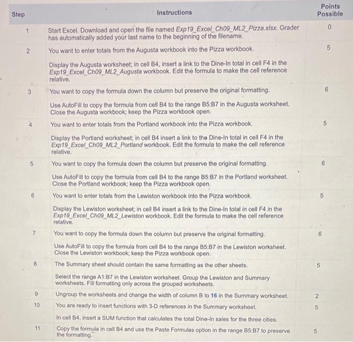
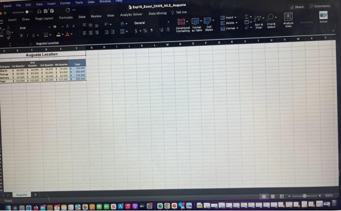
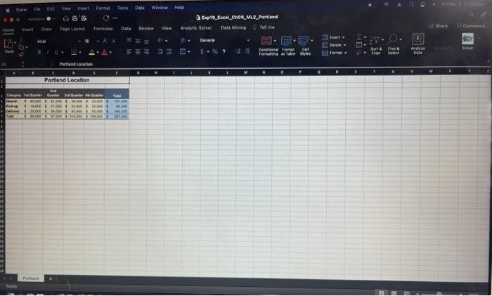
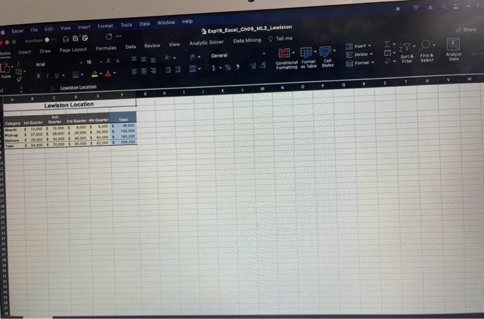
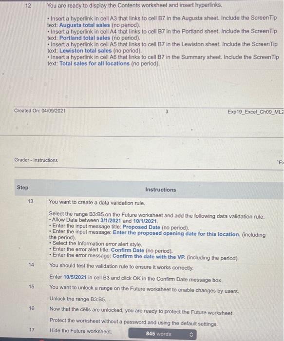
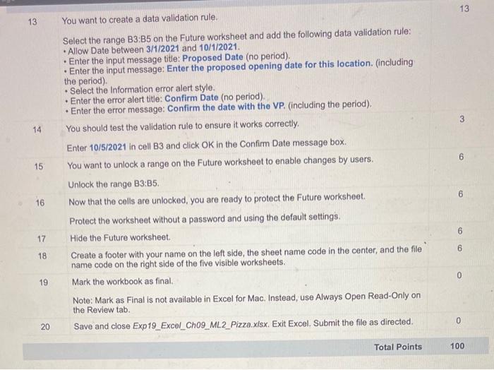
Step Instructions Possible 1 Start Excel. Download and open the file named Exp19_Excel_Ch09_ML2_Pizza.x/sx. Grader 0 has automatically added your last name to the beginning of the filename. 2. You want to enter totals from the Augusta workbook into the Pizza workbook. 5 Display the Augusta worksheet; in cell B4, insert a link to the Dine-In total in cell F4 in the Exp19_Excel_Ch09_ML2_Augusta workbook. Edit the formula to make the cell reference relative. 3 You want to copy the formula down the column but preserve the original formatting. 6 Use AutoFill to copy the formula from cell B4 to the range B5:B7 in the Augusta worksheet. Close the Augusta workbook; keep the Pizza workbook open. 4 You want to enter totals from the Portland workbook into the Pizza workbook. 5 Display the Portland worksheet; in cell B4 insert a link to the Dine-In total in cell F4 in the Exp19_Excel_Ch09_ML2_Portland workbook. Edit the formula to make the cell reference relative. 5 You want to copy the formula down the column but preserve the original formatting. 6 Use AutoFill to copy the formula from cell B4 to the range B5:B7 in the Portland worksheet. Close the Portland workbook; keep the Pizza workbook open. 6 You want to enter totals from the Lewiston workbook into the Pizza workbook. 5 Display the Lewiston worksheet; in cell B4 insert a link to the Dine-In total in cell F4 in the Exp19_Excel_Ch09_ML2_Lewiston workbook. Edit the formula to make the cell reference relative. 7 You want to copy the formula down the column but preserve the original formatting. 6 Use AutoFill to copy the formula from cell B4 to the range B5:B7 in the Lewiston worksheet. Close the Lewiston workbook; keep the Pizza workbook open. 8 The Summary sheet should contain the same formatting as the other sheets. 5 Select the range A1:B7 in the Lewiston worksheet. Group the Lewiston and Summary worksheets. Fill formatting only across the grouped worksheets. 9 Ungroup the worksheets and change the width of column B to 16 in the Summary worksheet. 2 10 You are ready to insert functions with 3-D references in the Summary worksheet. 5 In cell B4, insert a SUM function that calculates the total Dine-In sales for the three cities. 11 Copy the formula in cell B4 and use the Paste Formulas option in the range B5: B7 to preserve the formatting. 12 You are ready to display the Contents worksheet and insert hyperlinks. - Insert a hyperink in cell A3 that links to cell B7 in the Augusta sheot. Include the ScreenTip text: Augusta total sales (no period). - Insert a hyperlink in cell A4 that links to cell B7 in the Portland sheet. Include the ScreenTip text: Portland total sales (no period). - Insert a hyperlink in cell A5 that links to cell B7 in the Lewiston sheet. Include the ScreenTip text: Lewiston total sales (no period). - Insert a hyperlink in cell A6 that links to cell B7 in the Summary sheet. Include the ScreenTip text: Total sales for all locations (no period). Created On: 04/09/2021 3 Exp19_Excel_Ch09_ML2 Grader-Instructions Step Instructions 13 You want to create a data validation rule. Select the range B3:B5 on the Future worksheet and add the following data validation rule: - Allow Date between 3/1/2021 and 10/1/2021. - Enter the input message title: Proposed Date (no period). - Enter the input message: Enter the proposed opening date for this location. (including the period). - Select the Information error alert style. - Enter the error alert title: Confirm Date (no period). - Enter the error message: Confirm the date with the VP. (including the period). 14 You should test the validation rule to ensure it works correctly. Enter 10/5/2021 in cell B3 and click OK in the Confirm Date message box. 15 You want to unlock a range on the Future worksheet to enable changes by users. Unlock the range B3:B5. 16 Now that the cells are unlocked, you are ready to protect the Future worksheet. Protect the worksheet without a password and using the default setting5. 17 Hide the Future worksheet. 13 13 You want to create a data validation rule. Select the range B3:B5 on the Future worksheet and add the following data validation rule: - Allow Date between 3/1/2021 and 10/1/2021. - Enter the input message title: Proposed Date (no period). - Enter the input message: Enter the proposed opening date for this location. (including the period). - Select the Information error alert style. - Enter the error alert title: Confirm Date (no period). - Enter the error message: Confirm the date with the VP. (including the period). 14 You should test the validation rule to ensure it works correctly. Enter 10/5/2021 in cell B3 and click OK in the Confirm Date message box. 15 You want to unlock a range on the Future worksheet to enable changes by users. 6 Unlock the range B3:B5. 16 Now that the cells are unlocked, you are ready to protect the Future worksheet. 6 Protect the worksheet without a password and using the default settings. 6 17 Hide the Future worksheet. 18 Create a footer with your name on the left side, the sheet name code in the center, and the file 6 name code on the right side of the five visible worksheets. 19 Mark the workbook as final. 0 Note: Mark as Final is not available in Excel for Mac. Instead, use Always Open Read-Only on the Review tab. 20 Save and close Exp19_Excel_Ch09_ML2_Pizza.xlsx. Exit Excel. Submit the file as directed. 0 Total Points 100 Plans for Now Locations Step Instructions Possible 1 Start Excel. Download and open the file named Exp19_Excel_Ch09_ML2_Pizza.x/sx. Grader 0 has automatically added your last name to the beginning of the filename. 2. You want to enter totals from the Augusta workbook into the Pizza workbook. 5 Display the Augusta worksheet; in cell B4, insert a link to the Dine-In total in cell F4 in the Exp19_Excel_Ch09_ML2_Augusta workbook. Edit the formula to make the cell reference relative. 3 You want to copy the formula down the column but preserve the original formatting. 6 Use AutoFill to copy the formula from cell B4 to the range B5:B7 in the Augusta worksheet. Close the Augusta workbook; keep the Pizza workbook open. 4 You want to enter totals from the Portland workbook into the Pizza workbook. 5 Display the Portland worksheet; in cell B4 insert a link to the Dine-In total in cell F4 in the Exp19_Excel_Ch09_ML2_Portland workbook. Edit the formula to make the cell reference relative. 5 You want to copy the formula down the column but preserve the original formatting. 6 Use AutoFill to copy the formula from cell B4 to the range B5:B7 in the Portland worksheet. Close the Portland workbook; keep the Pizza workbook open. 6 You want to enter totals from the Lewiston workbook into the Pizza workbook. 5 Display the Lewiston worksheet; in cell B4 insert a link to the Dine-In total in cell F4 in the Exp19_Excel_Ch09_ML2_Lewiston workbook. Edit the formula to make the cell reference relative. 7 You want to copy the formula down the column but preserve the original formatting. 6 Use AutoFill to copy the formula from cell B4 to the range B5:B7 in the Lewiston worksheet. Close the Lewiston workbook; keep the Pizza workbook open. 8 The Summary sheet should contain the same formatting as the other sheets. 5 Select the range A1:B7 in the Lewiston worksheet. Group the Lewiston and Summary worksheets. Fill formatting only across the grouped worksheets. 9 Ungroup the worksheets and change the width of column B to 16 in the Summary worksheet. 2 10 You are ready to insert functions with 3-D references in the Summary worksheet. 5 In cell B4, insert a SUM function that calculates the total Dine-In sales for the three cities. 11 Copy the formula in cell B4 and use the Paste Formulas option in the range B5: B7 to preserve the formatting. 12 You are ready to display the Contents worksheet and insert hyperlinks. - Insert a hyperink in cell A3 that links to cell B7 in the Augusta sheot. Include the ScreenTip text: Augusta total sales (no period). - Insert a hyperlink in cell A4 that links to cell B7 in the Portland sheet. Include the ScreenTip text: Portland total sales (no period). - Insert a hyperlink in cell A5 that links to cell B7 in the Lewiston sheet. Include the ScreenTip text: Lewiston total sales (no period). - Insert a hyperlink in cell A6 that links to cell B7 in the Summary sheet. Include the ScreenTip text: Total sales for all locations (no period). Created On: 04/09/2021 3 Exp19_Excel_Ch09_ML2 Grader-Instructions Step Instructions 13 You want to create a data validation rule. Select the range B3:B5 on the Future worksheet and add the following data validation rule: - Allow Date between 3/1/2021 and 10/1/2021. - Enter the input message title: Proposed Date (no period). - Enter the input message: Enter the proposed opening date for this location. (including the period). - Select the Information error alert style. - Enter the error alert title: Confirm Date (no period). - Enter the error message: Confirm the date with the VP. (including the period). 14 You should test the validation rule to ensure it works correctly. Enter 10/5/2021 in cell B3 and click OK in the Confirm Date message box. 15 You want to unlock a range on the Future worksheet to enable changes by users. Unlock the range B3:B5. 16 Now that the cells are unlocked, you are ready to protect the Future worksheet. Protect the worksheet without a password and using the default setting5. 17 Hide the Future worksheet. 13 13 You want to create a data validation rule. Select the range B3:B5 on the Future worksheet and add the following data validation rule: - Allow Date between 3/1/2021 and 10/1/2021. - Enter the input message title: Proposed Date (no period). - Enter the input message: Enter the proposed opening date for this location. (including the period). - Select the Information error alert style. - Enter the error alert title: Confirm Date (no period). - Enter the error message: Confirm the date with the VP. (including the period). 14 You should test the validation rule to ensure it works correctly. Enter 10/5/2021 in cell B3 and click OK in the Confirm Date message box. 15 You want to unlock a range on the Future worksheet to enable changes by users. 6 Unlock the range B3:B5. 16 Now that the cells are unlocked, you are ready to protect the Future worksheet. 6 Protect the worksheet without a password and using the default settings. 6 17 Hide the Future worksheet. 18 Create a footer with your name on the left side, the sheet name code in the center, and the file 6 name code on the right side of the five visible worksheets. 19 Mark the workbook as final. 0 Note: Mark as Final is not available in Excel for Mac. Instead, use Always Open Read-Only on the Review tab. 20 Save and close Exp19_Excel_Ch09_ML2_Pizza.xlsx. Exit Excel. Submit the file as directed. 0 Total Points 100 Plans for Now Locations