I need help to sove it with explanation.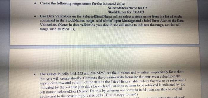

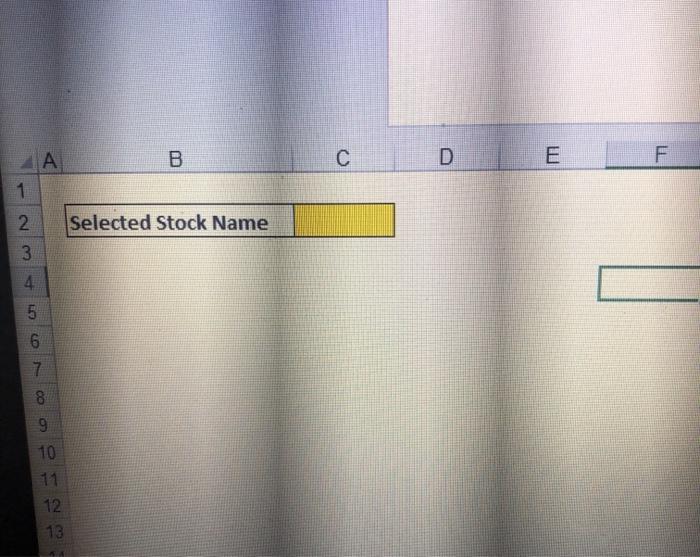
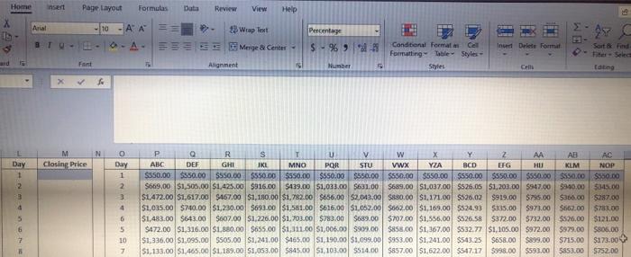
Create the following range names for the indicated cells: SelectedStockName for C2 StockNames for P3:AC3 Use Data Validation on the SelectedStockName cell to select a stock name from the list of stocks contained in the StockNames range. Add a brief Input Message and a brief Error Alert to the Data Validation. (Note: In data validation you should use cell name to indicate the range, not the cell range such as P3:AC3). The values in cells L4:L253 and M4:M253 are the x-values and y-values respectively for a chart that you will create shortly. Compute the y-values with formulae that retrieve a value from the appropriate row and column of the data in the Price History table, where the row to be retrieved is indicated by the x-value (the day) for each cell, and the column to be retrieved is indicated by the cell named selected Stock Name. Do this by entering one formula in M4 that can then be copied downward to the remaining y-value cells. (Do not copy format!). ibulue of Home Insert Page Layout Formulas Review View Help Arial Percentage 10 ' ' - Wrap Text OA-EESE Merge & Center Alignment $ -% 913 Inced Delete Format Sort & Find Conditional Format ca Formatting Theile Styles - Styles Font Number Crill Editing N M Closing Price Day 1 2 0 Day 1 2. 4 P R S T U V w X z AA AB AC ABC DEF GHI IKE MNO PQR STU Vwx BCD EFG HU KLM NOP $550.00 $350.00 $550.00 $550.00 $550.00 $550.00 $550.00 $550.00 $550.00 $550.00 $550.00 $550.00 $550,00 $550.00 5669.00 $1,500.00 51.425.00 $916.00 $439.00 $1,033.00 $631,00 5689.00 $1,037.00 $526.05 51,203.00 $947.00 $940.00 $345.00 $1.472.00 $1,617.00 $467.00 $1,180.00 $1,782,00 $656,00 $2,043.00 $830.00 $1,171.00 $536.02 $919.00 $795.00 $366.00 $287.00 $1,035.00 $740.00 $1,230.00 569 $1,581.00 $616.00 $1.052 $662.00 $1,169.00 $524.93 $335.00 $973.00 $662,00 $783.00 $1,483.00 $643.00 $607.00 $1,226.00 $1,700.00 $783.00 $689.00 $707.00 $1,556.00 $526.58 $372.00 $732.00 $526.00 $121.00 $472.00 $1,316.00 $1.880,00 $655.00 $1,111.00 $1,006,00 5909.00 $858.00 $1,367.00 $532.77 $1,105.00 $972.00 $979.00 $806,00 $1.336.00 $1,095.00 SS05.00 $1,241.00 $465,00 $1,190.00 $1,099.00 $953.00 $1,241,00 $543.25 $658.00 $899.00 $715.00 $173.00 $1.133.00 $1,465,00 $1. 189.00 51.053.00 5845.00 $1,103.00 $514.00 $857.00 $1,622.00 $547.17 $998.00 $593.00 $853.00 $752.00 6 5 10 7 7 Create the following range names for the indicated cells: SelectedStockName for C2 StockNames for P3:AC3 Use Data Validation on the SelectedStockName cell to select a stock name from the list of stocks contained in the StockNames range. Add a brief Input Message and a brief Error Alert to the Data Validation. (Note: In data validation you should use cell name to indicate the range, not the cell range such as P3:AC3). The values in cells L4:L253 and M4:M253 are the x-values and y-values respectively for a chart that you will create shortly. Compute the y-values with formulae that retrieve a value from the appropriate row and column of the data in the Price History table, where the row to be retrieved is indicated by the x-value (the day) for each cell, and the column to be retrieved is indicated by the cell named selected Stock Name. Do this by entering one formula in M4 that can then be copied downward to the remaining y-value cells. (Do not copy format!). ibulue of Home Insert Page Layout Formulas Review View Help Arial Percentage 10 ' ' - Wrap Text OA-EESE Merge & Center Alignment $ -% 913 Inced Delete Format Sort & Find Conditional Format ca Formatting Theile Styles - Styles Font Number Crill Editing N M Closing Price Day 1 2 0 Day 1 2. 4 P R S T U V w X z AA AB AC ABC DEF GHI IKE MNO PQR STU Vwx BCD EFG HU KLM NOP $550.00 $350.00 $550.00 $550.00 $550.00 $550.00 $550.00 $550.00 $550.00 $550.00 $550.00 $550.00 $550,00 $550.00 5669.00 $1,500.00 51.425.00 $916.00 $439.00 $1,033.00 $631,00 5689.00 $1,037.00 $526.05 51,203.00 $947.00 $940.00 $345.00 $1.472.00 $1,617.00 $467.00 $1,180.00 $1,782,00 $656,00 $2,043.00 $830.00 $1,171.00 $536.02 $919.00 $795.00 $366.00 $287.00 $1,035.00 $740.00 $1,230.00 569 $1,581.00 $616.00 $1.052 $662.00 $1,169.00 $524.93 $335.00 $973.00 $662,00 $783.00 $1,483.00 $643.00 $607.00 $1,226.00 $1,700.00 $783.00 $689.00 $707.00 $1,556.00 $526.58 $372.00 $732.00 $526.00 $121.00 $472.00 $1,316.00 $1.880,00 $655.00 $1,111.00 $1,006,00 5909.00 $858.00 $1,367.00 $532.77 $1,105.00 $972.00 $979.00 $806,00 $1.336.00 $1,095.00 SS05.00 $1,241.00 $465,00 $1,190.00 $1,099.00 $953.00 $1,241,00 $543.25 $658.00 $899.00 $715.00 $173.00 $1.133.00 $1,465,00 $1. 189.00 51.053.00 5845.00 $1,103.00 $514.00 $857.00 $1,622.00 $547.17 $998.00 $593.00 $853.00 $752.00 6 5 10 7 7