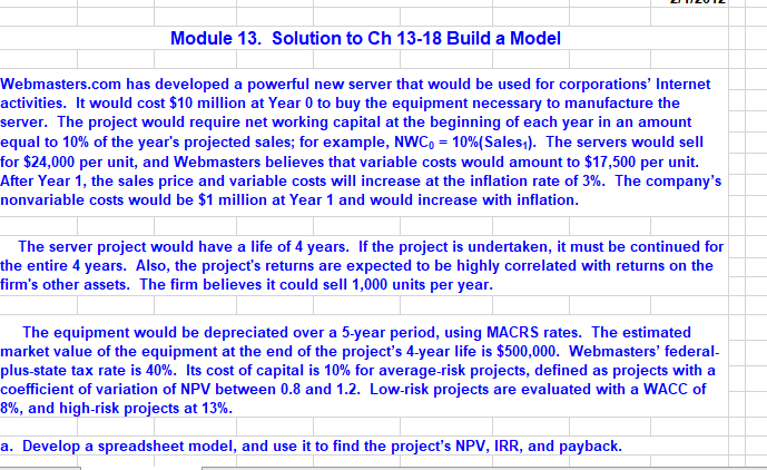
i need help with part 7 section c and d show formulas please.

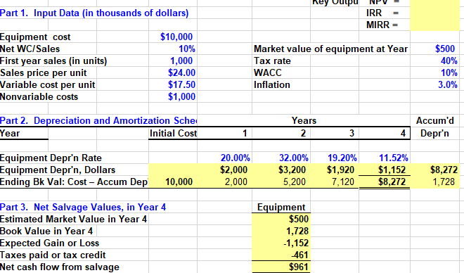
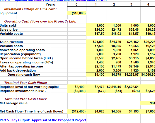
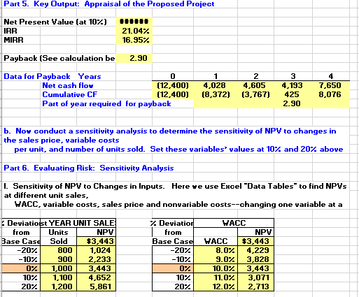
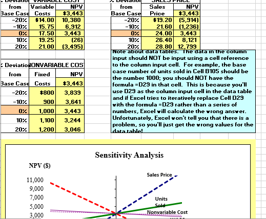
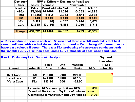
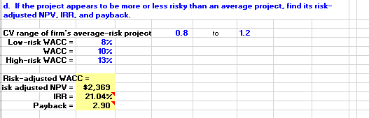
Module 13. Solution to Ch 13-18 Build a Model Webmasters.com has developed a powerful new server that would be used for corporations' Internet activities. It would cost $10 million at Year 0 to buy the equipment necessary to manufacture the server. The project would require net working capital at the beginning of each year in an amount equal to 10% of the year's projected sales; for example, NWC,-10%(Sales). The servers would sell for $24,000 per unit, and Webmasters believes that variable costs would amount to $17,500 per unit. After Year 1, the sales price and variable costs will increase at the inflation rate of 3%. The company's nonvariable costs would be $1 million at Year 1 and would increase with inflation The server project would have a life of 4 years. If the project is undertaken, it must be continued for the entire 4 years. Also, the project's returns are expected to be highly correlated with returns on the firm's other assets. The firm believes it could sell 1,000 units per year The equipment would be depreciated over a 5-year period, using MACRS rates. The estimated market value of the equipment at the end of the project's 4-year life is $500,000. Webmasters' federal plus-state tax rate is 40%. Its cost of capital is 10% for average-risk projects, defined as projects with a coefficient of variation of NPV between 0.8 and 1.2. Low-risk projects are evaluated with a WACC of 8%, and high-risk projects at 13% a. Develop a spreadsheet model, and use it to find the project's NPV, IRR, and payback Part 1. Input Data (in thousands of dollars) IRR MIRR $10,000 10% 1,000 $24.00 $17.50 $1,000 Equipment cost Net WC/Sales First year sales (in units) Sales price per unit Variable cost per unit Nonvariable costs $500 40% 10% 3.0% Market value of equipment at Year Tax rate WACC Inflation Accum'd 4Depr'n Part 2. Depreciation and Amortization Sche Year Years Initial Cost 2 32.00% 5,200 11.52% Equipment Depr'n Rate Equipment Depr'n, Dollars Ending Bk Val: Cost- Accum De 20.00% $2,000 2,000 19.20% $3,200 $1,920 $1,152 $8,272 1,728 7,120 $8,272 10,000 Part 3. Net Salvage Values, in Year 4 Estimated Market Value in Year 4 Book Value in Year 4 Expected Gain or Loss Taxes paid or tax credit Net cash flow from salvage Equipment $500 1,728 1,152 461 $961 Years Investment Outlays at Time Zero: Equipment ($10,000) Operating Cash Flows over the Project's Life Units sold Sales price Variable costs 1,000 1,000 $24.00 $24.72 $25.46 $26.23 $17.50 $18.03 $18.57 $19.12 1,000 1,000 $24,000 $24,720 $25,462 $26,225 17,500 18,025 18,566 9,123 1,061 1,093 1.152 $3,500 $2,465 $3,915 $4,858 Sales revenue Variable costs Nonvariable operating costs Depreciation (equipment) Oper. income before taxes (EBIT) Taxes on operating income (40%) After-tax operating income Add back depreciation 1,000 2,000 1,030 1,920 1,400 1,94 986 $2,100 $1,479 $2,349 $2,915 1,152 $4,100 $4,679 $4,268.97 $4,066.80 2,000 1,920 Operating cash flow Terminal Year Cash Flows: $2,472 $2,546.16 $2,622.54 Required level of net working capital $2,400 ($2,400) ($72) ($74) Required investment in NWC (S76) $2,623 Terminal Year Cash Flows: 961 Net salvage value Net Cash Flow (Time line of cash flows) ($12,400) $4,028S4,605$4,193 7,650 Part 5. Key Output: Appraisal of the Proposed Project Part 5. Key Output: Appraisal of the Proposed Project IRR 21.04% 16.95% MIRR Payback (See calculation be Data for Payback Years 2.90 0 Net cash flow Cumulative CF Part of year required for payback (12.400) 4,0284,605 4.193 7,650 8.076 (12.400) (8,372) (3,767) 425 2.90 b. Nor conduct a sensitivity analysis to determine the sensitivity of NP the sales price, variable costs to changes in per unit, and number of units sold. Set these variables, values at 10% and 20% above Part 6. Evaluating Risk: Sensitivity Analysis I. Sensitivity of NP to Changes in Inputs. Heree use Excel "Data Tables to find NPVs at different unit sales HACC. variable costs. sales price and nonvariable costs--changing one variable at a Deviatiolst YEAR UNIT SALE NPV $3,443 % Deviato HACC Units Base Case Sold NPV Base CaseHACC$3,443 8.0%| 4,229 9.0%| 3,828 10.0% | 3,443 11.0% 3,071 12.0%| 2,713 20% 10% 800 1,000 20%) 1.200 1,024 900 2.233 0% | | 3,443 10% | 1,100| 4,652 5,861 20% 10% 0% 10% 20% NPV sts$3,443 Sales NPV $3,443 $19.20 (5,914) 21.60(1.236) 24.003,443 26.40 8,121 28.80 12,799 fromVariable Base Case Costs Base Cas 20%! $14.00 10,380 -10% | 15-75 6,912 0% | 17.50 3,443 19.25 21.00 20% 10% 0% 10% 20% 10% | 20%| (26) (3,495) input should NOT be input using a cell reference to the column input cell For example, the base case number of units sold in Cell B105 should be the number 1000; you should NOT have the formula- D29 in that cell. This is because you'l use D29 as the column input cell in the data table and if Excel tries to iteratively replace Cell D29 ith the formula D29 rather than a series of numbers, Encelill calculate the rong ans er Unfortunately. Excel on't tell you that there is a problem, so you'll just get the rong values for the DeviatioHONVARIABLE COS Fixed NPy Base Case Costs -20% 10% 0% | 10% | 20% | $8003,839 9003,641 1,000 | 3,443 1,100| 3,244 1,200 3,046 Sensitivity Analysis NPV (S) Sales Price 11,000 9,000 7,000 5,000 3.000 Units variable Cost Deviatio from Base Cas NPV at Different Deviations from Base Sales Variable Price Nonvariable Cost Cost!Unit Units Sold HACC 10% 0% 10% (1236)6,912 3,443 3,443 2.233 3.443 3,6413,828 3,4433,443 3.2443,071 3,0462.713 (26)4.652 12.7993,495)5,861 8.121 20% Range $18,712$4,837 C. Now conduct a scenario analysis. Assume that there is a 25% probability that best case conditions, with each of the variables discussed in Part b being 20% better than its base-case value, will occur. There is a 25% probability of worst-case conditions, with the variables 20% worse than base, and a 50% probability of base-case conditions Part 7. Evaluating Risk: Scenario Analysis Squared Deviation Sales Unit Sales Variable Costs Scenario Probabilit Price NPV robabilit Best Case Base Case Horst Case 25% *28.80 1,200 50% *24.00 1,000 800 $14.00 $17.50 $21.00 25% $19.20 $18 Expected NPV- sum. prob times NPV Standard Deviation-Sq Root of column H sum Coefficient of Variation Std Dev Expec 0.00 d. If the project appears to be more or less risky than an average project, find its risk- adjusted NPV. IRR, and payback. 1.2 0.8 to CV range of firm's average-risk project 8% 10% 13% Low-risk WACC = HACC High-risk WACC Risk-adjusted WACC $2.369 21.04% isk adjusted NPV- IRR- Payback 2.90 Module 13. Solution to Ch 13-18 Build a Model Webmasters.com has developed a powerful new server that would be used for corporations' Internet activities. It would cost $10 million at Year 0 to buy the equipment necessary to manufacture the server. The project would require net working capital at the beginning of each year in an amount equal to 10% of the year's projected sales; for example, NWC,-10%(Sales). The servers would sell for $24,000 per unit, and Webmasters believes that variable costs would amount to $17,500 per unit. After Year 1, the sales price and variable costs will increase at the inflation rate of 3%. The company's nonvariable costs would be $1 million at Year 1 and would increase with inflation The server project would have a life of 4 years. If the project is undertaken, it must be continued for the entire 4 years. Also, the project's returns are expected to be highly correlated with returns on the firm's other assets. The firm believes it could sell 1,000 units per year The equipment would be depreciated over a 5-year period, using MACRS rates. The estimated market value of the equipment at the end of the project's 4-year life is $500,000. Webmasters' federal plus-state tax rate is 40%. Its cost of capital is 10% for average-risk projects, defined as projects with a coefficient of variation of NPV between 0.8 and 1.2. Low-risk projects are evaluated with a WACC of 8%, and high-risk projects at 13% a. Develop a spreadsheet model, and use it to find the project's NPV, IRR, and payback Part 1. Input Data (in thousands of dollars) IRR MIRR $10,000 10% 1,000 $24.00 $17.50 $1,000 Equipment cost Net WC/Sales First year sales (in units) Sales price per unit Variable cost per unit Nonvariable costs $500 40% 10% 3.0% Market value of equipment at Year Tax rate WACC Inflation Accum'd 4Depr'n Part 2. Depreciation and Amortization Sche Year Years Initial Cost 2 32.00% 5,200 11.52% Equipment Depr'n Rate Equipment Depr'n, Dollars Ending Bk Val: Cost- Accum De 20.00% $2,000 2,000 19.20% $3,200 $1,920 $1,152 $8,272 1,728 7,120 $8,272 10,000 Part 3. Net Salvage Values, in Year 4 Estimated Market Value in Year 4 Book Value in Year 4 Expected Gain or Loss Taxes paid or tax credit Net cash flow from salvage Equipment $500 1,728 1,152 461 $961 Years Investment Outlays at Time Zero: Equipment ($10,000) Operating Cash Flows over the Project's Life Units sold Sales price Variable costs 1,000 1,000 $24.00 $24.72 $25.46 $26.23 $17.50 $18.03 $18.57 $19.12 1,000 1,000 $24,000 $24,720 $25,462 $26,225 17,500 18,025 18,566 9,123 1,061 1,093 1.152 $3,500 $2,465 $3,915 $4,858 Sales revenue Variable costs Nonvariable operating costs Depreciation (equipment) Oper. income before taxes (EBIT) Taxes on operating income (40%) After-tax operating income Add back depreciation 1,000 2,000 1,030 1,920 1,400 1,94 986 $2,100 $1,479 $2,349 $2,915 1,152 $4,100 $4,679 $4,268.97 $4,066.80 2,000 1,920 Operating cash flow Terminal Year Cash Flows: $2,472 $2,546.16 $2,622.54 Required level of net working capital $2,400 ($2,400) ($72) ($74) Required investment in NWC (S76) $2,623 Terminal Year Cash Flows: 961 Net salvage value Net Cash Flow (Time line of cash flows) ($12,400) $4,028S4,605$4,193 7,650 Part 5. Key Output: Appraisal of the Proposed Project Part 5. Key Output: Appraisal of the Proposed Project IRR 21.04% 16.95% MIRR Payback (See calculation be Data for Payback Years 2.90 0 Net cash flow Cumulative CF Part of year required for payback (12.400) 4,0284,605 4.193 7,650 8.076 (12.400) (8,372) (3,767) 425 2.90 b. Nor conduct a sensitivity analysis to determine the sensitivity of NP the sales price, variable costs to changes in per unit, and number of units sold. Set these variables, values at 10% and 20% above Part 6. Evaluating Risk: Sensitivity Analysis I. Sensitivity of NP to Changes in Inputs. Heree use Excel "Data Tables to find NPVs at different unit sales HACC. variable costs. sales price and nonvariable costs--changing one variable at a Deviatiolst YEAR UNIT SALE NPV $3,443 % Deviato HACC Units Base Case Sold NPV Base CaseHACC$3,443 8.0%| 4,229 9.0%| 3,828 10.0% | 3,443 11.0% 3,071 12.0%| 2,713 20% 10% 800 1,000 20%) 1.200 1,024 900 2.233 0% | | 3,443 10% | 1,100| 4,652 5,861 20% 10% 0% 10% 20% NPV sts$3,443 Sales NPV $3,443 $19.20 (5,914) 21.60(1.236) 24.003,443 26.40 8,121 28.80 12,799 fromVariable Base Case Costs Base Cas 20%! $14.00 10,380 -10% | 15-75 6,912 0% | 17.50 3,443 19.25 21.00 20% 10% 0% 10% 20% 10% | 20%| (26) (3,495) input should NOT be input using a cell reference to the column input cell For example, the base case number of units sold in Cell B105 should be the number 1000; you should NOT have the formula- D29 in that cell. This is because you'l use D29 as the column input cell in the data table and if Excel tries to iteratively replace Cell D29 ith the formula D29 rather than a series of numbers, Encelill calculate the rong ans er Unfortunately. Excel on't tell you that there is a problem, so you'll just get the rong values for the DeviatioHONVARIABLE COS Fixed NPy Base Case Costs -20% 10% 0% | 10% | 20% | $8003,839 9003,641 1,000 | 3,443 1,100| 3,244 1,200 3,046 Sensitivity Analysis NPV (S) Sales Price 11,000 9,000 7,000 5,000 3.000 Units variable Cost Deviatio from Base Cas NPV at Different Deviations from Base Sales Variable Price Nonvariable Cost Cost!Unit Units Sold HACC 10% 0% 10% (1236)6,912 3,443 3,443 2.233 3.443 3,6413,828 3,4433,443 3.2443,071 3,0462.713 (26)4.652 12.7993,495)5,861 8.121 20% Range $18,712$4,837 C. Now conduct a scenario analysis. Assume that there is a 25% probability that best case conditions, with each of the variables discussed in Part b being 20% better than its base-case value, will occur. There is a 25% probability of worst-case conditions, with the variables 20% worse than base, and a 50% probability of base-case conditions Part 7. Evaluating Risk: Scenario Analysis Squared Deviation Sales Unit Sales Variable Costs Scenario Probabilit Price NPV robabilit Best Case Base Case Horst Case 25% *28.80 1,200 50% *24.00 1,000 800 $14.00 $17.50 $21.00 25% $19.20 $18 Expected NPV- sum. prob times NPV Standard Deviation-Sq Root of column H sum Coefficient of Variation Std Dev Expec 0.00 d. If the project appears to be more or less risky than an average project, find its risk- adjusted NPV. IRR, and payback. 1.2 0.8 to CV range of firm's average-risk project 8% 10% 13% Low-risk WACC = HACC High-risk WACC Risk-adjusted WACC $2.369 21.04% isk adjusted NPV- IRR- Payback 2.90