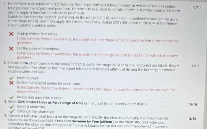
I need help with the questions I got wrong. Step by step instructions would be helpful.

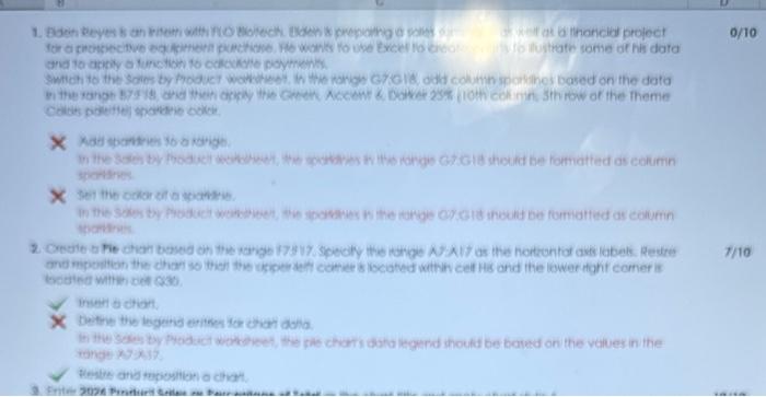
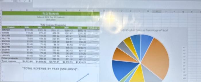
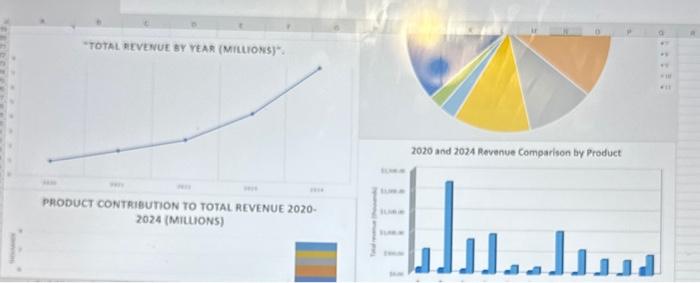
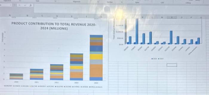
ard 10 akchy o tunction 16 colckate poymenth. X Nad stantren 10 a rigige. siculises X sel the cokar ef a soaneis. thandentith boted white cen caso. ment de chart. tange x817 Weithe anid reposhtion o char. teakether) "Totki firvicue ar veak (Gruions). "Total nevenue BY YeAR (MiLLONS)". PHODUCT CONT1UTION TO TOTAL REVENUE 20202024 (MIULNS) 1. Bden Reyes is an intem with FLO Biotech. Eden is preparing a sales summary, as well as a financial project for a prospective equipment purchase. He wants to use Excel to create charts to llustrate some of his data and to apply a function to colculate payments. Switch to the Sales by Product worksheet. In the range G7:G18, add column sparklines bosed on the data In the range B7:F18, and then opply the Green, Accent 6 , Dorker 25% (10th column, 5 th row of the Theme Calors polette) spandine color. Add sparklines to a range. In the Sales by Product workheet, the spaklines in the range G7iGl8 should be formatted as column sparilines. Set the color of o sparkine. In the Sales by Product worksheet, the sparkines in the range G7G18 should be formatted as column spankines. 2. Create a Pie chart bosed on the range F7:F17. Specify the range A7:AI7 as the harizontal axis labels. Resize and reposition the chart so that the upperteft comer is located within cell Hb and the lower-fght comer is located within cel Q30. Insert a chari. Define the legend entries for chart data. In the Sales by Product workheet, the ple chart's data legend should be based on the values in the range A7A17 Resize and reposition a chart. 3. Enter 2024 Product Sales as Percentage of Total as the chart title and apply chart style 6 . Insert a chart titie. 10/10 Change the chart style. 4. Create a 2-D Line chart based on the range 818:F18. Modify the chart by changing the horizontal axls labets to use the range B6:F6. Enter Total Revenue by Year (Milions) as the chart title, and resize and reposition the chart so that the uppetteft comer is located within cell A20 and the lower dabt camer 10. Change the background color of the plot area to White, Background 1 and then change the backgrounc color of the chart area to Green, Accent 6 , Lighter 80% (10th column, 2nd row in the Theme Colors palettel. X Change the fill color of the plot area of a chart. In the Sales by Product worksheet, the 3-D clustered column chart's plof area should be formatfed using the White, Background I fil color. X Change the fill color of the chart area of a chart. In the Sales by Product worksheet, the 3-D clustered column chart's chart area should be formatted using the Green. Accent 6 , Lighter 80% fill color. ard 10 akchy o tunction 16 colckate poymenth. X Nad stantren 10 a rigige. siculises X sel the cokar ef a soaneis. thandentith boted white cen caso. ment de chart. tange x817 Weithe anid reposhtion o char. teakether) "Totki firvicue ar veak (Gruions). "Total nevenue BY YeAR (MiLLONS)". PHODUCT CONT1UTION TO TOTAL REVENUE 20202024 (MIULNS) 1. Bden Reyes is an intem with FLO Biotech. Eden is preparing a sales summary, as well as a financial project for a prospective equipment purchase. He wants to use Excel to create charts to llustrate some of his data and to apply a function to colculate payments. Switch to the Sales by Product worksheet. In the range G7:G18, add column sparklines bosed on the data In the range B7:F18, and then opply the Green, Accent 6 , Dorker 25% (10th column, 5 th row of the Theme Calors polette) spandine color. Add sparklines to a range. In the Sales by Product workheet, the spaklines in the range G7iGl8 should be formatted as column sparilines. Set the color of o sparkine. In the Sales by Product worksheet, the sparkines in the range G7G18 should be formatted as column spankines. 2. Create a Pie chart bosed on the range F7:F17. Specify the range A7:AI7 as the harizontal axis labels. Resize and reposition the chart so that the upperteft comer is located within cell Hb and the lower-fght comer is located within cel Q30. Insert a chari. Define the legend entries for chart data. In the Sales by Product workheet, the ple chart's data legend should be based on the values in the range A7A17 Resize and reposition a chart. 3. Enter 2024 Product Sales as Percentage of Total as the chart title and apply chart style 6 . Insert a chart titie. 10/10 Change the chart style. 4. Create a 2-D Line chart based on the range 818:F18. Modify the chart by changing the horizontal axls labets to use the range B6:F6. Enter Total Revenue by Year (Milions) as the chart title, and resize and reposition the chart so that the uppetteft comer is located within cell A20 and the lower dabt camer 10. Change the background color of the plot area to White, Background 1 and then change the backgrounc color of the chart area to Green, Accent 6 , Lighter 80% (10th column, 2nd row in the Theme Colors palettel. X Change the fill color of the plot area of a chart. In the Sales by Product worksheet, the 3-D clustered column chart's plof area should be formatfed using the White, Background I fil color. X Change the fill color of the chart area of a chart. In the Sales by Product worksheet, the 3-D clustered column chart's chart area should be formatted using the Green. Accent 6 , Lighter 80% fill color
