Question: I need the code in R studio, to find the results of table 5.7 5.6 MISSING DATA In many problems, some variables will be unrecorded
I need the code in R studio, to find the results of table 5.7


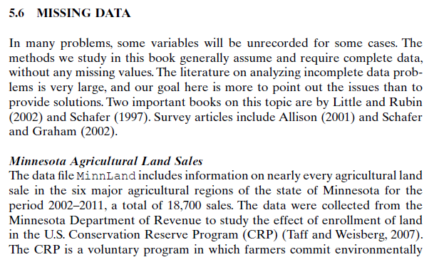
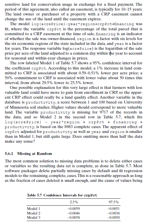
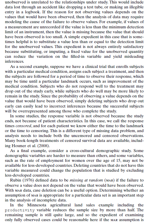
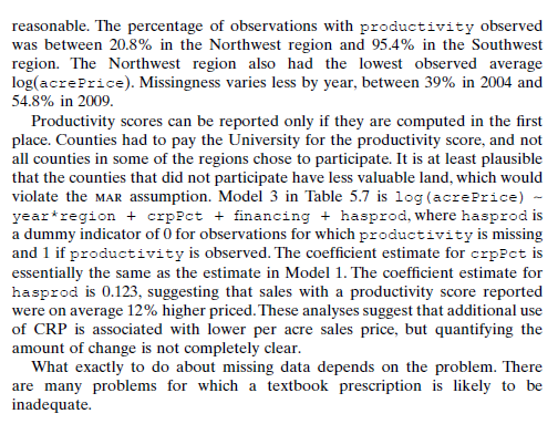
5.6 MISSING DATA In many problems, some variables will be unrecorded for some cases. The methods we study in this book generally assume and require complete data, without any missing values. The literature on analyzing incomplete data prob- lems is very large, and our goal here is more to point out the issues than to provide solutions. Two important books on this topic are by Little and Rubin (2002) and Schafer (1997). Survey articles include Allison (2001) and Schafer and Graham (2002). Minnesota Agricultural Land Sales The data file MinnLand includes information on nearly every agricultural land sale in the six major agricultural regions of the state of Minnesota for the period 2002-2011, a total of 18,700 sales. The data were collected from the Minnesota Department of Revenue to study the effect of enrollment of land in the U.S. Conservation Reserve Program (CRP) (Taff and Weisberg, 2007). The CRP is a voluntary program in which farmers commit environmentally sensitive land for conservation usage in exchange for a fixed payment. The period of this agreement, also called an easement, is typically for 10-15 years. The land owner or purchaser of a property with a CRP easement cannot change the use of the land until the easement expires. The model log (acrePrice)-year region+crpct+financing was fit, where the variable crpect is the percentage of the total parcel that is committed to a CRP easement at the time of sale, financing is an indicator of whether the sale was owner-financed, region is a factor with six levels for the six economic regions of the state included in the data, and year is a factor for years. The response variable log(acrePrice) is the logarithm of the sale price per acre of the land adjusted to a common day within the year to account for seasonal and within-year changes in prices. The row labeled Model 1 of Table 5.7 shows a 95% confidence interval for the coefficient crprct. According to this model, a 1% increase in land com- mitted to CRP is associated with about 0.59-0.51% lower per acre price; a 50% commitment to CRP is associated with lower value about 50 times this interval, from about 29.5% lower to 25.5% lower. One possible explanation for this very large effect is that farmers with less valuable land could have more to gain from enrollment in CRP, so the appar- ent CRP effect could really be a land quality effect. Another variable in the database is productivity, a score between 1 and 100 based on University of Minnesota soil studies. Higher values should correspond to more valuable land. The variable productivity is missing for 9717 of the records in the data, and so Model 2 in the second row in Table 5.7, which fits log (acre Price) year*region + crprct + financing + productivity, is based on the 8983 complete cases. The apparent effect of crpect adjusted for productivity as well as year and region is smaller than in Model 1, but still quite large. Does omitting more than half the data make any sense? 5.6.1 Missing at Random The most common solution to missing data problems is to delete either cases or variables so the resulting data set is complete, as done in Table 5.7. Most software packages delete partially missing cases by default and fit regression models to the remaining, complete, cases. This is a reasonable approach as long as the fraction of cases deleted is small enough, and the cause of values being Table 5.7 Confidence Intervals for crpPct 2.5% Model 1 -0.0059 Model 2 -0.0046 Model 3 -0.0058 97.5% -0.0051 -0.0036 -0.0050 unobserved is unrelated to the relationships under study. This would include data lost through an accident like dropping a test tube, or making an illegible entry in a logbook. If the reason for not observing values depends on the values that would have been observed, then the analysis of data may require modeling the cause of the failure to observe values. For example, if values of a measurement are unrecorded if the value is less than the minimum detection limit of an instrument, then the value is missing because the value that should have been observed is too small. A simple expedient in this case that is some- times helpful is to substitute a value less than or equal to the detection limit for the unobserved values. This expedient is not always entirely satisfactory because substituting, or imputing, a fixed value for the unobserved quantity can reduce the variation on the filled-in variable and yield misleading inferences. As a second example, suppose we have a clinical trial that enrolls subjects with a particular medical condition, assigns each subject a treatment, and then the subjects are followed for a period of time to observe their response, which may be time until a particular landmark occurs, such as improvement of the medical condition. Subjects who do not respond well to the treatment may drop out of the study early, while subjects who do well may be more likely to remain in the study. Since the probability of observing a value depends on the value that would have been observed, simply deleting subjects who drop out early can easily lead to incorrect inferences because the successful subjects will be overrepresented among those who complete the study. In some studies, the response variable is not observed because the study ends, not because of patient characteristics. In this case, we call the response times censored, and for each patient we know either the time to the landmark or the time to censoring. This is a different type of missing data problem, and analysis needs to include both the uncensored and censored observations. Many book-length treatments of censored survival data are available, includ- ing Hosmer et al. (2008). As a final example, consider a cross-cultural demographic study. Some demographic variables are harder to measure than others, and some variables, such as the rate of employment for women over the age of 15, may not be available for less-developed countries. Deleting countries that do not have this variable measured could change the population that is studied by excluding less-developed countries. Rubin (1976) defined data to be missing at random (MAR) if the failure to observe a value does not depend on the value that would have been observed. With MAR data, case deletion can be a useful option. Determining whether an assumption of MAR is appropriate for a particular data set is an important step in the analysis of incomplete data. In the Minnesota agricultural land sales example including the productivity variable reduces the sample size by more than half. The remaining sample is still quite large, and so the expedient of examining only fully observed cases could be reasonable here if the MAR assumption is reasonable. The percentage of observations with productivity observed was between 20.8% in the Northwest region and 95.4% in the Southwest region. The Northwest region also had the lowest observed average log(acre Price). Missingness varies less by year, between 39% in 2004 and 54.8% in 2009. Productivity scores can be reported only if they are computed in the first place. Counties had to pay the University for the productivity score, and not all counties in some of the regions chose to participate. It is at least plausible that the counties that did not participate have less valuable land, which would violate the MAR assumption. Model 3 in Table 5.7 is log (acrePrice) - year*region + crpPct + financing + hasprod, where hasprod is a dummy indicator of 0 for observations for which productivity is missing and 1 if productivity is observed. The coefficient estimate for crpPct is essentially the same as the estimate in Model 1. The coefficient estimate for hasprod is 0.123, suggesting that sales with a productivity score reported were on average 12% higher priced. These analyses suggest that additional use of CRP is associated with lower per acre sales price, but quantifying the amount of change is not completely clear. What exactly to do about missing data depends on the problem. There are many problems for which a textbook prescription is likely to be inadequate. 5.6 MISSING DATA In many problems, some variables will be unrecorded for some cases. The methods we study in this book generally assume and require complete data, without any missing values. The literature on analyzing incomplete data prob- lems is very large, and our goal here is more to point out the issues than to provide solutions. Two important books on this topic are by Little and Rubin (2002) and Schafer (1997). Survey articles include Allison (2001) and Schafer and Graham (2002). Minnesota Agricultural Land Sales The data file MinnLand includes information on nearly every agricultural land sale in the six major agricultural regions of the state of Minnesota for the period 2002-2011, a total of 18,700 sales. The data were collected from the Minnesota Department of Revenue to study the effect of enrollment of land in the U.S. Conservation Reserve Program (CRP) (Taff and Weisberg, 2007). The CRP is a voluntary program in which farmers commit environmentally sensitive land for conservation usage in exchange for a fixed payment. The period of this agreement, also called an easement, is typically for 10-15 years. The land owner or purchaser of a property with a CRP easement cannot change the use of the land until the easement expires. The model log (acrePrice)-year region+crpct+financing was fit, where the variable crpect is the percentage of the total parcel that is committed to a CRP easement at the time of sale, financing is an indicator of whether the sale was owner-financed, region is a factor with six levels for the six economic regions of the state included in the data, and year is a factor for years. The response variable log(acrePrice) is the logarithm of the sale price per acre of the land adjusted to a common day within the year to account for seasonal and within-year changes in prices. The row labeled Model 1 of Table 5.7 shows a 95% confidence interval for the coefficient crprct. According to this model, a 1% increase in land com- mitted to CRP is associated with about 0.59-0.51% lower per acre price; a 50% commitment to CRP is associated with lower value about 50 times this interval, from about 29.5% lower to 25.5% lower. One possible explanation for this very large effect is that farmers with less valuable land could have more to gain from enrollment in CRP, so the appar- ent CRP effect could really be a land quality effect. Another variable in the database is productivity, a score between 1 and 100 based on University of Minnesota soil studies. Higher values should correspond to more valuable land. The variable productivity is missing for 9717 of the records in the data, and so Model 2 in the second row in Table 5.7, which fits log (acre Price) year*region + crprct + financing + productivity, is based on the 8983 complete cases. The apparent effect of crpect adjusted for productivity as well as year and region is smaller than in Model 1, but still quite large. Does omitting more than half the data make any sense? 5.6.1 Missing at Random The most common solution to missing data problems is to delete either cases or variables so the resulting data set is complete, as done in Table 5.7. Most software packages delete partially missing cases by default and fit regression models to the remaining, complete, cases. This is a reasonable approach as long as the fraction of cases deleted is small enough, and the cause of values being Table 5.7 Confidence Intervals for crpPct 2.5% Model 1 -0.0059 Model 2 -0.0046 Model 3 -0.0058 97.5% -0.0051 -0.0036 -0.0050 unobserved is unrelated to the relationships under study. This would include data lost through an accident like dropping a test tube, or making an illegible entry in a logbook. If the reason for not observing values depends on the values that would have been observed, then the analysis of data may require modeling the cause of the failure to observe values. For example, if values of a measurement are unrecorded if the value is less than the minimum detection limit of an instrument, then the value is missing because the value that should have been observed is too small. A simple expedient in this case that is some- times helpful is to substitute a value less than or equal to the detection limit for the unobserved values. This expedient is not always entirely satisfactory because substituting, or imputing, a fixed value for the unobserved quantity can reduce the variation on the filled-in variable and yield misleading inferences. As a second example, suppose we have a clinical trial that enrolls subjects with a particular medical condition, assigns each subject a treatment, and then the subjects are followed for a period of time to observe their response, which may be time until a particular landmark occurs, such as improvement of the medical condition. Subjects who do not respond well to the treatment may drop out of the study early, while subjects who do well may be more likely to remain in the study. Since the probability of observing a value depends on the value that would have been observed, simply deleting subjects who drop out early can easily lead to incorrect inferences because the successful subjects will be overrepresented among those who complete the study. In some studies, the response variable is not observed because the study ends, not because of patient characteristics. In this case, we call the response times censored, and for each patient we know either the time to the landmark or the time to censoring. This is a different type of missing data problem, and analysis needs to include both the uncensored and censored observations. Many book-length treatments of censored survival data are available, includ- ing Hosmer et al. (2008). As a final example, consider a cross-cultural demographic study. Some demographic variables are harder to measure than others, and some variables, such as the rate of employment for women over the age of 15, may not be available for less-developed countries. Deleting countries that do not have this variable measured could change the population that is studied by excluding less-developed countries. Rubin (1976) defined data to be missing at random (MAR) if the failure to observe a value does not depend on the value that would have been observed. With MAR data, case deletion can be a useful option. Determining whether an assumption of MAR is appropriate for a particular data set is an important step in the analysis of incomplete data. In the Minnesota agricultural land sales example including the productivity variable reduces the sample size by more than half. The remaining sample is still quite large, and so the expedient of examining only fully observed cases could be reasonable here if the MAR assumption is reasonable. The percentage of observations with productivity observed was between 20.8% in the Northwest region and 95.4% in the Southwest region. The Northwest region also had the lowest observed average log(acre Price). Missingness varies less by year, between 39% in 2004 and 54.8% in 2009. Productivity scores can be reported only if they are computed in the first place. Counties had to pay the University for the productivity score, and not all counties in some of the regions chose to participate. It is at least plausible that the counties that did not participate have less valuable land, which would violate the MAR assumption. Model 3 in Table 5.7 is log (acrePrice) - year*region + crpPct + financing + hasprod, where hasprod is a dummy indicator of 0 for observations for which productivity is missing and 1 if productivity is observed. The coefficient estimate for crpPct is essentially the same as the estimate in Model 1. The coefficient estimate for hasprod is 0.123, suggesting that sales with a productivity score reported were on average 12% higher priced. These analyses suggest that additional use of CRP is associated with lower per acre sales price, but quantifying the amount of change is not completely clear. What exactly to do about missing data depends on the problem. There are many problems for which a textbook prescription is likely to be inadequate
Step by Step Solution
There are 3 Steps involved in it

Get step-by-step solutions from verified subject matter experts


