I specifically need help on #12 for SimNet Excel 2021 Ch4 Independet Project 4-4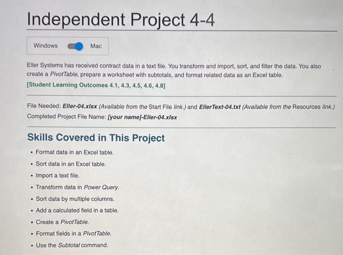

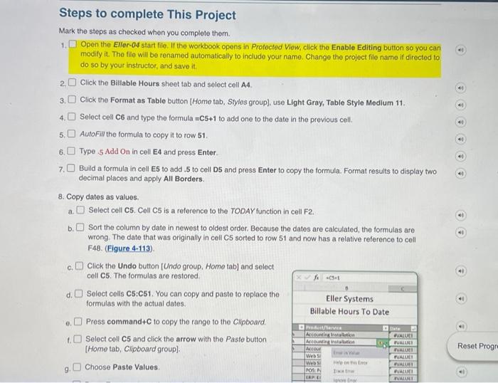
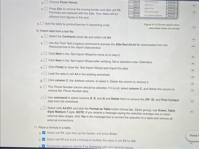
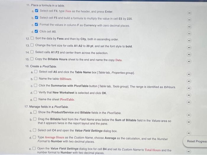
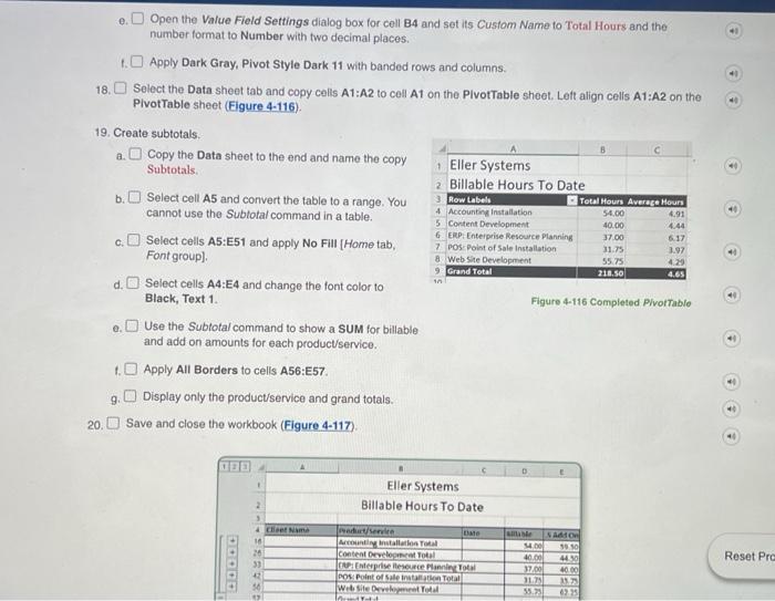
Eller Systems has received contract data in a text file. You transform and import, sort, and filter the data. You also create a PivotTable, prepare a worksheet with subtotals, and format related data as an Excel table. [Student Learning Outcomes 4.1, 4.3, 4.5, 4.6, 4.8] File Needed: Eller-04.xIsx (Available from the Start File link.) and EllerText-04.txt (Avallable from the Resources link.) Completed Project File Name: [your name]-Eller-04.x/sx Skills Covered in This Project - Format data in an Excel table. - Sort data in an Excel table. - Import a text file. - Transform data in Power Query. - Sort data by multiple columns. - Add a calculated field in a table. - Create a PivotTable. - Format fields in a PivotTable. - Use the Subtotal command. Steps to complete This Project Mark the steps as checked when you complete them. 1. Open the Eller-04 start file. If the workbook opens in Prolocted Viow, click the Enable Editing button so you can modify it. The file will be renamed automatically to include your name. Change the project filo name if directed to do so by your instructor, and save it. 2. Click the Billable Hours sheet tab and select cell A4. 3. Click the Format as Table button [Home tab, Styles group], use Light Gray, Table Style Medium 11. 4. Select cell C6 and type the formula =C5+1 to add one to the date in the previous cell. 5. Autofiil the formula to copy it to row 51. 6. Type .5 Add On in cell E4 and press Enter. 7. Build a formula in cell E5 to add .5 to cell D5 and press Enter to copy the formula. Format results to display two decimal places and apply All Borders. 8. Copy dates as values. a. Select cell C5. Cell C5 is a reference to the TODAY function in cell F2. b. Sort the column by date in newest to oldest order. Because the dates are calculated, the formulas are wrong. The date that was originally in cell C5 sorted to row 51 and now has a relative reference to cell F48. (Figure 4-113). c. Click the Undo button [Undo group. Home tab] and select cell C5. The formulas are restored. d. Select cells C5:C51. You can copy and paste to replace the formulas with the actual dates. e. Press command +C to copy the range to the Clipboard. t. Select cell C5 and click the arrow with the Paste button [Home tab, Clipboard group]. 9. Choose Paste Values. 9. Choose Paste Values. h. Press Esc to remove the moving border and click cell C5. Formulas are replaced with the date. Your dates will be different from figures in this text. 9. Sort the table by product/service in ascending order. Figure 4-113 Errors resuit when calculated dates are sorted 10. Import data from a text file. a. Select the Contracts sheet tab and select cell A4. b. Use the From Text (Legacy) command to previow the EllerText-04.txt file downloaded from the Resources link in the Import Data window. c. Click Next in the Text Import Wizard to move on to step 2. d. Click Next in the Toxt Import Wizard after verifying Tab is selected under Delimiters. e. Click Finish to close the Text import Wizard and import the data. f. Load the data to cell A4 in the existing worksheet. 9. Click column C, the Addross column, to select it. Delete the column to remove it. h. The Phone Number column should be selected. If it is not, solect column C, and delete the column to remove the Phone Number data. 1. Use command to select columns D, E, and G and Delete them to remove the ZIP, ID, and First Contact data from the worksheet. 1. Solect cells A4:E31 and click the Format as Table button [Home tab, Styles group], use Green, Table Style Medium 7 style. NOTE: If you receive a message saying the selection overiaps one or more external data ranges, click Yes in the message box to convert the selection to a table and remove all external connections. 11. Place a formuta in a table. a. Solect cell F4, type Fees as the header, and pross Enter. b. Select cell F5 and build a formula to multiply the value in cell E5 by 225 . a. Format the values in column F as Currency with zero decimal places. 16. Create a PivorTable. a. Select cell A5 and click the Table Name box [Table tab, Properties group]. b. Name the table tblHours: c. Click the Summarize with PivotTable button [Table tab, Tools group]. The range is identified as tbiHours. d. Verify that New Worksheet is selected and click OK. e. Name the sheet PivotTable. 17. Manage fields in a ProtTable. a. Show the Product/Service and Billable fields in the PrvotTable. b. Drag the Billable field from the Fleld Name area below the Sum of Blllable field in the Values area so that it appears twice in the report layout and the pane. c. Select cell CA and open the Value Flold Sottings dialog box. d. Type Average Hours as the Custom Name, choose Average as the calculation, and set the Number Format to Number with two decimal places. e. Open the Value Fleld Settings dialog box for cell B4 and set its Custom Name to Total Hours and the number format to Number with two decimal places. e. Open the Value Field Settings dialog box for cell B4 and set its Custom Name to Total Hours and the number format to Number with two decimal places. 1. Apply Dark Gray, Pivot Style Dark 11 with banded rows and columns. 18. Select the Data sheet tab and copy cells A1:A2 to cell A1 on the PlvotTable sheet. Left align cells A1:A2 on the Pivot Table sheet (Eigure 4-116). 19. Create subtotals. a. Copy the Data sheet to the end and name the copy Subtotals. b. Select cell A5 and convert the table to a range. You cannot use the Subtotal command in a table. c. Select cells A5:E51 and apply No Fill [Home tab, Font group]. d. Select cells A4:E4 and change the font color to Black, Text 1. Figure 4-116 Completed PlvorTablo e. Use the Sublotal command to show a Sum for billable and add on amounts for each product/service. t. Apply All Borders to cells A56:E57. 9. Display only the product/service and grand totals. 20. Save and close the workbook (Figure 4-117). Eller Systems has received contract data in a text file. You transform and import, sort, and filter the data. You also create a PivotTable, prepare a worksheet with subtotals, and format related data as an Excel table. [Student Learning Outcomes 4.1, 4.3, 4.5, 4.6, 4.8] File Needed: Eller-04.xIsx (Available from the Start File link.) and EllerText-04.txt (Avallable from the Resources link.) Completed Project File Name: [your name]-Eller-04.x/sx Skills Covered in This Project - Format data in an Excel table. - Sort data in an Excel table. - Import a text file. - Transform data in Power Query. - Sort data by multiple columns. - Add a calculated field in a table. - Create a PivotTable. - Format fields in a PivotTable. - Use the Subtotal command. Steps to complete This Project Mark the steps as checked when you complete them. 1. Open the Eller-04 start file. If the workbook opens in Prolocted Viow, click the Enable Editing button so you can modify it. The file will be renamed automatically to include your name. Change the project filo name if directed to do so by your instructor, and save it. 2. Click the Billable Hours sheet tab and select cell A4. 3. Click the Format as Table button [Home tab, Styles group], use Light Gray, Table Style Medium 11. 4. Select cell C6 and type the formula =C5+1 to add one to the date in the previous cell. 5. Autofiil the formula to copy it to row 51. 6. Type .5 Add On in cell E4 and press Enter. 7. Build a formula in cell E5 to add .5 to cell D5 and press Enter to copy the formula. Format results to display two decimal places and apply All Borders. 8. Copy dates as values. a. Select cell C5. Cell C5 is a reference to the TODAY function in cell F2. b. Sort the column by date in newest to oldest order. Because the dates are calculated, the formulas are wrong. The date that was originally in cell C5 sorted to row 51 and now has a relative reference to cell F48. (Figure 4-113). c. Click the Undo button [Undo group. Home tab] and select cell C5. The formulas are restored. d. Select cells C5:C51. You can copy and paste to replace the formulas with the actual dates. e. Press command +C to copy the range to the Clipboard. t. Select cell C5 and click the arrow with the Paste button [Home tab, Clipboard group]. 9. Choose Paste Values. 9. Choose Paste Values. h. Press Esc to remove the moving border and click cell C5. Formulas are replaced with the date. Your dates will be different from figures in this text. 9. Sort the table by product/service in ascending order. Figure 4-113 Errors resuit when calculated dates are sorted 10. Import data from a text file. a. Select the Contracts sheet tab and select cell A4. b. Use the From Text (Legacy) command to previow the EllerText-04.txt file downloaded from the Resources link in the Import Data window. c. Click Next in the Text Import Wizard to move on to step 2. d. Click Next in the Toxt Import Wizard after verifying Tab is selected under Delimiters. e. Click Finish to close the Text import Wizard and import the data. f. Load the data to cell A4 in the existing worksheet. 9. Click column C, the Addross column, to select it. Delete the column to remove it. h. The Phone Number column should be selected. If it is not, solect column C, and delete the column to remove the Phone Number data. 1. Use command to select columns D, E, and G and Delete them to remove the ZIP, ID, and First Contact data from the worksheet. 1. Solect cells A4:E31 and click the Format as Table button [Home tab, Styles group], use Green, Table Style Medium 7 style. NOTE: If you receive a message saying the selection overiaps one or more external data ranges, click Yes in the message box to convert the selection to a table and remove all external connections. 11. Place a formuta in a table. a. Solect cell F4, type Fees as the header, and pross Enter. b. Select cell F5 and build a formula to multiply the value in cell E5 by 225 . a. Format the values in column F as Currency with zero decimal places. 16. Create a PivorTable. a. Select cell A5 and click the Table Name box [Table tab, Properties group]. b. Name the table tblHours: c. Click the Summarize with PivotTable button [Table tab, Tools group]. The range is identified as tbiHours. d. Verify that New Worksheet is selected and click OK. e. Name the sheet PivotTable. 17. Manage fields in a ProtTable. a. Show the Product/Service and Billable fields in the PrvotTable. b. Drag the Billable field from the Fleld Name area below the Sum of Blllable field in the Values area so that it appears twice in the report layout and the pane. c. Select cell CA and open the Value Flold Sottings dialog box. d. Type Average Hours as the Custom Name, choose Average as the calculation, and set the Number Format to Number with two decimal places. e. Open the Value Fleld Settings dialog box for cell B4 and set its Custom Name to Total Hours and the number format to Number with two decimal places. e. Open the Value Field Settings dialog box for cell B4 and set its Custom Name to Total Hours and the number format to Number with two decimal places. 1. Apply Dark Gray, Pivot Style Dark 11 with banded rows and columns. 18. Select the Data sheet tab and copy cells A1:A2 to cell A1 on the PlvotTable sheet. Left align cells A1:A2 on the Pivot Table sheet (Eigure 4-116). 19. Create subtotals. a. Copy the Data sheet to the end and name the copy Subtotals. b. Select cell A5 and convert the table to a range. You cannot use the Subtotal command in a table. c. Select cells A5:E51 and apply No Fill [Home tab, Font group]. d. Select cells A4:E4 and change the font color to Black, Text 1. Figure 4-116 Completed PlvorTablo e. Use the Sublotal command to show a Sum for billable and add on amounts for each product/service. t. Apply All Borders to cells A56:E57. 9. Display only the product/service and grand totals. 20. Save and close the workbook (Figure 4-117)