I want to use MATLAB to solve tutorial 2.1. My question is about computational neuroscience.

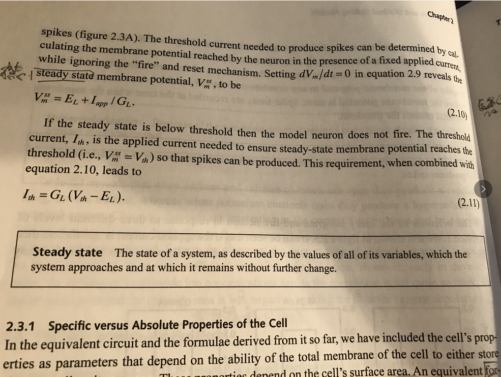
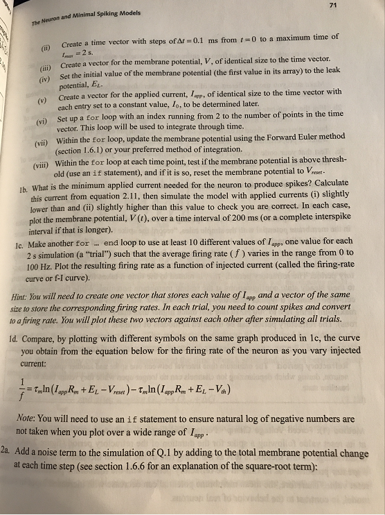
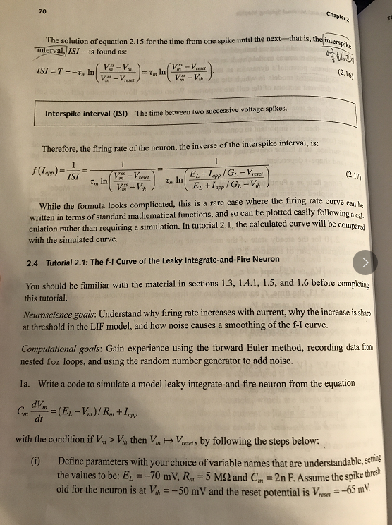
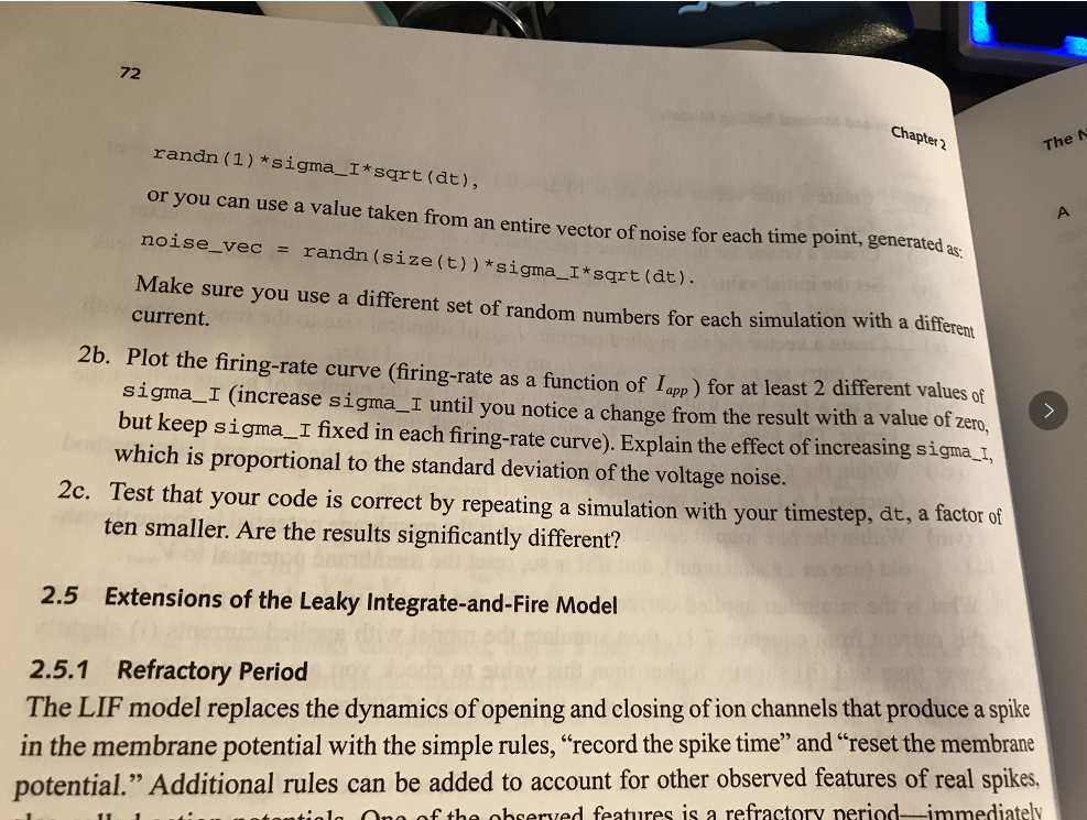
Chapter spikes (figure 2.3A). The threshold current needed to produce spikes can be determined by cl culating the membrane potential reached by the neuron in while ignoring the "fire" and reset mechanism. Setting dVm/d plied current 0 in equation 2.9 reveals the the presence of a fixed ap 1 Isteady state membrane potential, V to be (2.10 If the steady state is below threshold then the model neuron does not fire. The threshold current, lus, is the applied current needed to ensure steady-state membrane potential reaches the threshold (i.e., VIP ) so that spikes can be produced. This requirement, when combined with equation 2.10, leads to la = GL (yah-EL). Steady state The state of a system, as described by the values of all of its variables, which the system approaches and at which it remains without further change. 2.3.1 Specific versus Absolute Properties of the Cell arameters that depend on the ability of the total membrane of the cell to either store rtias denend on the cell's surface area. An equivalent for nt circuit and the formulae derived from it so far, we have included the cell's prop- erties as p 71 Neuron and Minimal Splking Models i) Create a time vector with steps of Ar 0.1 ms from0 to a maximum time of Create a vector for the membrane potential, V, of identical size to the time vector Set the initial value of the membrane potential (the first value in its array) to the leak potential, E Create a vector for the applied current, Iapp, of identical size to the time vector with ch entry set to a constant value, lo, to be determined later Set up a for loop with an index running from 2 to the number of points in the time vector. This loop will be used to integrate through time. ea (vi) (vi) Within the for loop, update the membrane potential using the Forward Euler method. (section 1.6.1) or your preferred method of integration Within the for loop at each time point, test if the membrane potential is above thresh- old (use an if statement), and if it is so, reset the membrane potential to Vresei b. What is the minimum applied current needed for the neuron to produce spikes? Calculate this current from equation 2.11, then simulate the model with applied currents () slightly lower than and (ii) slightly higher than this value to check you are correct. In each case, plot the membrane potential, V (1), over a time interval of 200 ms (or a complete interspike interval if that is longer). Ic. Make another for end loop to use at least 10 different values of app, one value for each 2 s simulation (a "trial") such that the average firing rate (f) varies in the range from 0 to 100 Hz. Plot the resulting firing rate as a function of injected current (called the firing-rate curve or f-I curve). Hint: You will need to create one vector that stores each value of lap and a vector of the same size to store the corresponding firing rates. In each trial, you need to count spikes and convert to afiring rate. You will plot these two vectors against each other after simulating all trials. Id. Compare, by plotting with different symbols on the same graph produced in 1c, the curve you obtain from the equation below for the firing rate of the neuron as you vary injected current: Note: You will need to use an i f statement to ensure natural log of negative numbers are not taken when you plot over a wide range of Lapp 2a. Add a noise term to the simulation of Q.1 by adding to the total membrane potential change at each time step (see section 1.6.6 for an explanation of the square-root term): 70 Chapter 2 The solution of equation 2.15 for the time from one spike until the next -that is, thcjinterspi, TntervalyIS1-is found (2.16 The time between two successive vo ltage spikes. Interspike interval (ISI) Therefore, the firing rate of the neuron, the inverse of the interspike interval, is app ISI (2.17 While the formula looks complicated, this is a rare case where the firing rate curve can ha written in terms of standard mathematical functions, and so can be plotted easily followi culation rather than requiring a simulation. In tutorial 2.1, the calculated curve will be with the simulated curve a cal. compared 2.4 Tutorial 2.1: The f-1 Curve of the Leaky Integrate-and-Fire Neuron You should be familiar with the material in sections 1.3, 1.4.1, 1.5, and 1.6 before completing this tutorial. Neuroscience goals: Understand why firing rate increases with current, why the increase is sharp at threshold in the LIF model, and how noise causes a smoothing of the f-I curve. Computational goals: Gain experience using the forward Euler method, recording data from nested for loops, and using the random number generator to add noise. la. Write a code to simulate a model leaky integrate-and-fire neuron from the equation dt o bd Define parameters with your choice of variable names that are understandable, settit the values to be: EL = old for the neuron is at V, -50 mV and the reset potential is Vres6 parameters with your choice of variable names that are understandable. set -5 M and C (i) 70 mV, R = 2n F. Assume the spike the 72 Chapter The N randn (1) *sigma_I* sqrt (dt), or you can use a value taken from an entire vector of noise for each time noise-vec randn ( size (t))*sigma-1 * sqrt (dt). = Make sure you use a different set of random numbers for each simulation with a different current. 2b. Plot the firing-rate curve (firing-rate as a function of Lapp) for at least 2 different values of sigma_I (increase sigma I until you notice a change from the result with a value of zero but keep sigma_I fixed in each firing-rate curve). Explain the effect of increasing sigma t, which is proportional to the standard deviation of the voltage noise. 2c. Test that your code is correct by repeating a simulation with your timestep, at, a factor of ten smaller. Are the results significantly different? 2.5 Extensions of the Leaky Integrate-and-Fire Model 2.5.1 Refractory Period The LIF model replaces the dynamics of opening and closing ofion channels that produce a spike in the membrane potential with the simple rules, "record the spike time" and '"reset the membrane potential." Additional rules can be added to account for other observed features of real spikes. antilo Ome of the hserved features is a refractory neriod--immediatelv Chapter spikes (figure 2.3A). The threshold current needed to produce spikes can be determined by cl culating the membrane potential reached by the neuron in while ignoring the "fire" and reset mechanism. Setting dVm/d plied current 0 in equation 2.9 reveals the the presence of a fixed ap 1 Isteady state membrane potential, V to be (2.10 If the steady state is below threshold then the model neuron does not fire. The threshold current, lus, is the applied current needed to ensure steady-state membrane potential reaches the threshold (i.e., VIP ) so that spikes can be produced. This requirement, when combined with equation 2.10, leads to la = GL (yah-EL). Steady state The state of a system, as described by the values of all of its variables, which the system approaches and at which it remains without further change. 2.3.1 Specific versus Absolute Properties of the Cell arameters that depend on the ability of the total membrane of the cell to either store rtias denend on the cell's surface area. An equivalent for nt circuit and the formulae derived from it so far, we have included the cell's prop- erties as p 71 Neuron and Minimal Splking Models i) Create a time vector with steps of Ar 0.1 ms from0 to a maximum time of Create a vector for the membrane potential, V, of identical size to the time vector Set the initial value of the membrane potential (the first value in its array) to the leak potential, E Create a vector for the applied current, Iapp, of identical size to the time vector with ch entry set to a constant value, lo, to be determined later Set up a for loop with an index running from 2 to the number of points in the time vector. This loop will be used to integrate through time. ea (vi) (vi) Within the for loop, update the membrane potential using the Forward Euler method. (section 1.6.1) or your preferred method of integration Within the for loop at each time point, test if the membrane potential is above thresh- old (use an if statement), and if it is so, reset the membrane potential to Vresei b. What is the minimum applied current needed for the neuron to produce spikes? Calculate this current from equation 2.11, then simulate the model with applied currents () slightly lower than and (ii) slightly higher than this value to check you are correct. In each case, plot the membrane potential, V (1), over a time interval of 200 ms (or a complete interspike interval if that is longer). Ic. Make another for end loop to use at least 10 different values of app, one value for each 2 s simulation (a "trial") such that the average firing rate (f) varies in the range from 0 to 100 Hz. Plot the resulting firing rate as a function of injected current (called the firing-rate curve or f-I curve). Hint: You will need to create one vector that stores each value of lap and a vector of the same size to store the corresponding firing rates. In each trial, you need to count spikes and convert to afiring rate. You will plot these two vectors against each other after simulating all trials. Id. Compare, by plotting with different symbols on the same graph produced in 1c, the curve you obtain from the equation below for the firing rate of the neuron as you vary injected current: Note: You will need to use an i f statement to ensure natural log of negative numbers are not taken when you plot over a wide range of Lapp 2a. Add a noise term to the simulation of Q.1 by adding to the total membrane potential change at each time step (see section 1.6.6 for an explanation of the square-root term): 70 Chapter 2 The solution of equation 2.15 for the time from one spike until the next -that is, thcjinterspi, TntervalyIS1-is found (2.16 The time between two successive vo ltage spikes. Interspike interval (ISI) Therefore, the firing rate of the neuron, the inverse of the interspike interval, is app ISI (2.17 While the formula looks complicated, this is a rare case where the firing rate curve can ha written in terms of standard mathematical functions, and so can be plotted easily followi culation rather than requiring a simulation. In tutorial 2.1, the calculated curve will be with the simulated curve a cal. compared 2.4 Tutorial 2.1: The f-1 Curve of the Leaky Integrate-and-Fire Neuron You should be familiar with the material in sections 1.3, 1.4.1, 1.5, and 1.6 before completing this tutorial. Neuroscience goals: Understand why firing rate increases with current, why the increase is sharp at threshold in the LIF model, and how noise causes a smoothing of the f-I curve. Computational goals: Gain experience using the forward Euler method, recording data from nested for loops, and using the random number generator to add noise. la. Write a code to simulate a model leaky integrate-and-fire neuron from the equation dt o bd Define parameters with your choice of variable names that are understandable, settit the values to be: EL = old for the neuron is at V, -50 mV and the reset potential is Vres6 parameters with your choice of variable names that are understandable. set -5 M and C (i) 70 mV, R = 2n F. Assume the spike the 72 Chapter The N randn (1) *sigma_I* sqrt (dt), or you can use a value taken from an entire vector of noise for each time noise-vec randn ( size (t))*sigma-1 * sqrt (dt). = Make sure you use a different set of random numbers for each simulation with a different current. 2b. Plot the firing-rate curve (firing-rate as a function of Lapp) for at least 2 different values of sigma_I (increase sigma I until you notice a change from the result with a value of zero but keep sigma_I fixed in each firing-rate curve). Explain the effect of increasing sigma t, which is proportional to the standard deviation of the voltage noise. 2c. Test that your code is correct by repeating a simulation with your timestep, at, a factor of ten smaller. Are the results significantly different? 2.5 Extensions of the Leaky Integrate-and-Fire Model 2.5.1 Refractory Period The LIF model replaces the dynamics of opening and closing ofion channels that produce a spike in the membrane potential with the simple rules, "record the spike time" and '"reset the membrane potential." Additional rules can be added to account for other observed features of real spikes. antilo Ome of the hserved features is a refractory neriod--immediatelv