ill thumbs up who ever can help me with this. i posted what my code looks like up to this point with the instructions

i have no experience with coding and will appreciate any help

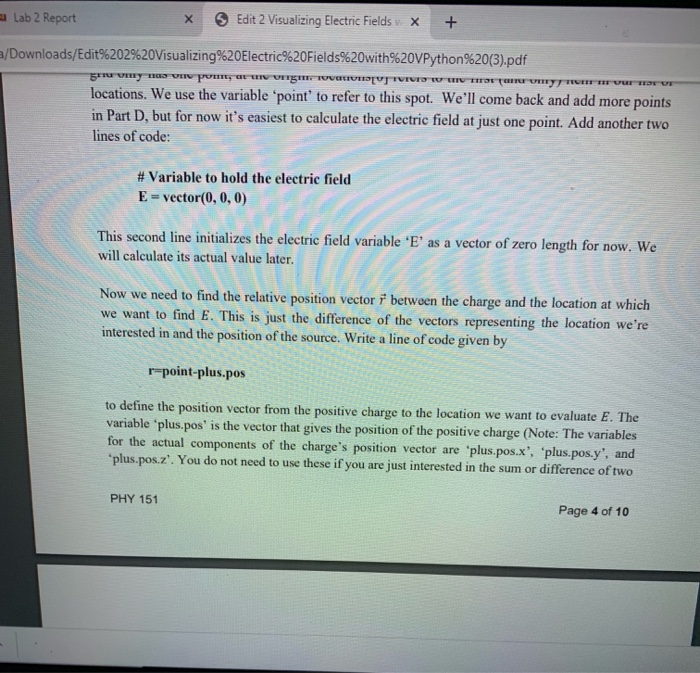
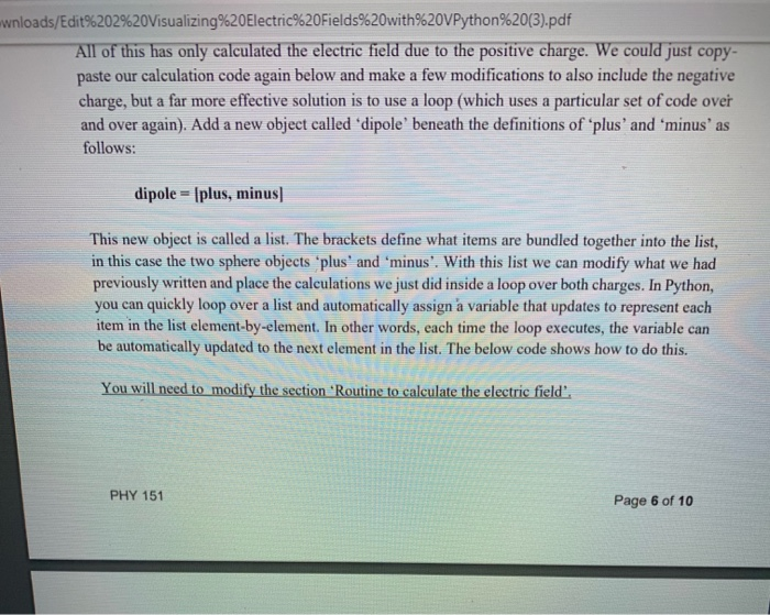
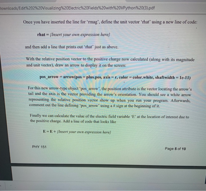
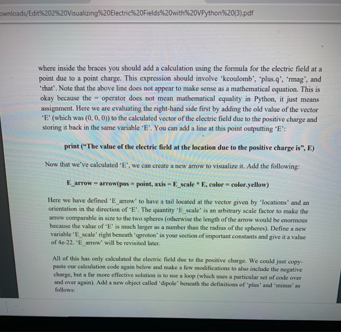
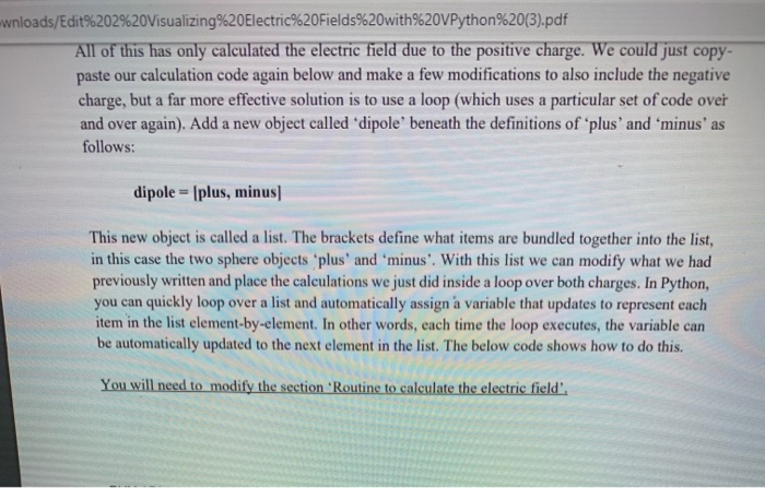
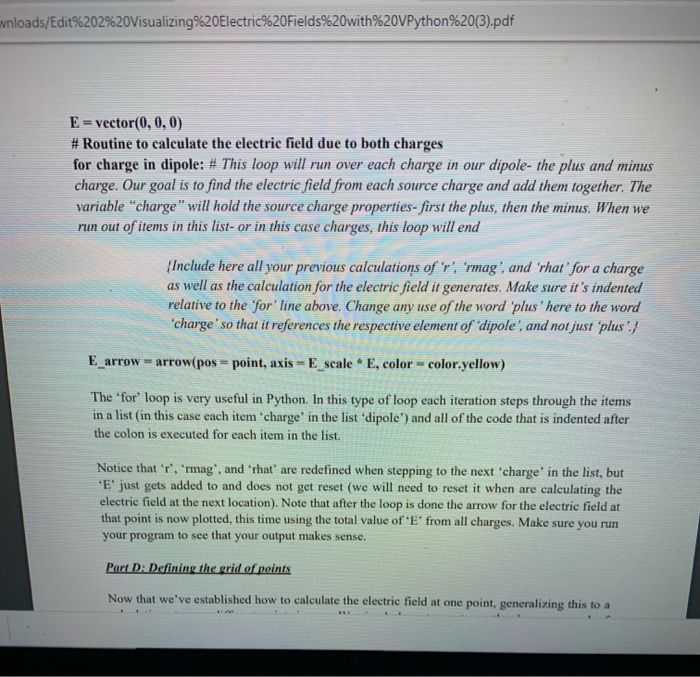
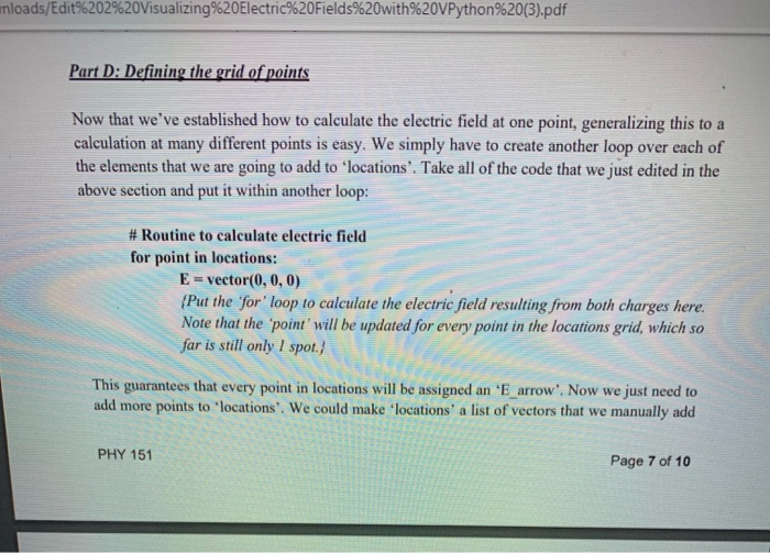
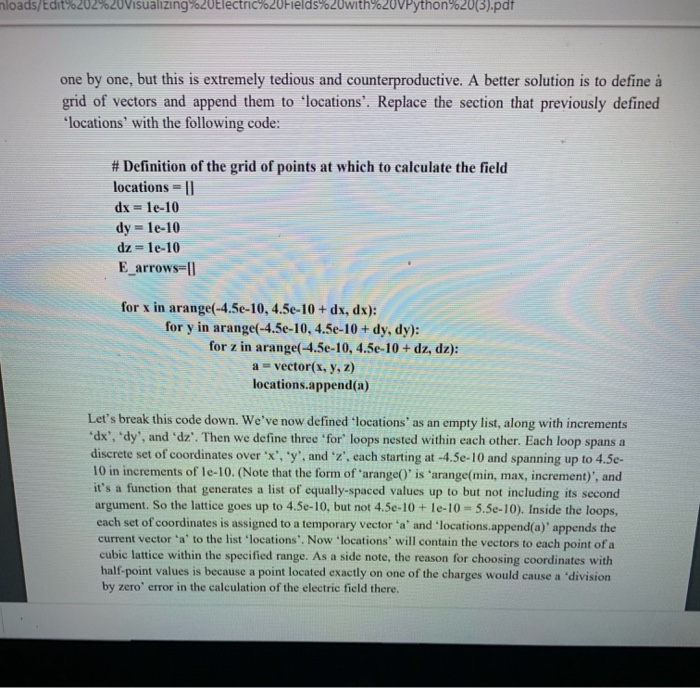
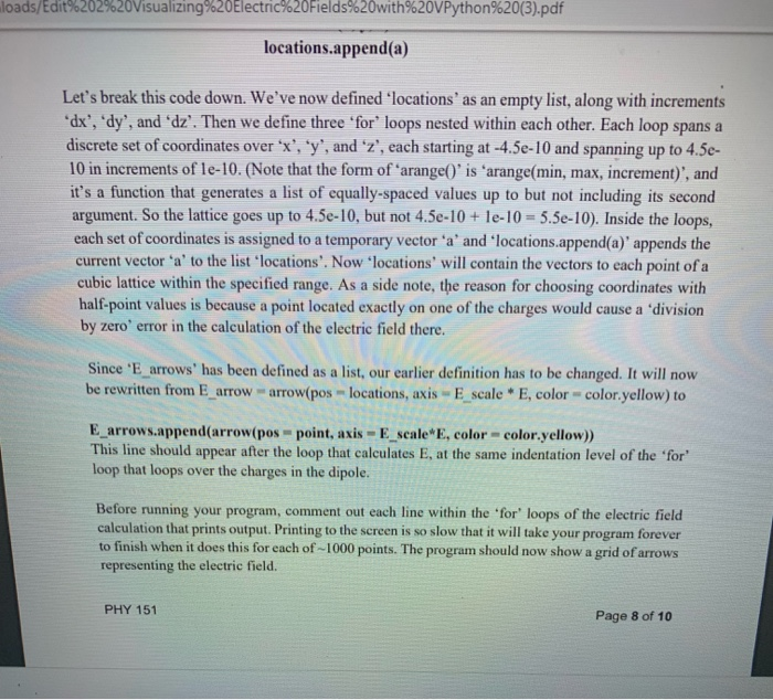
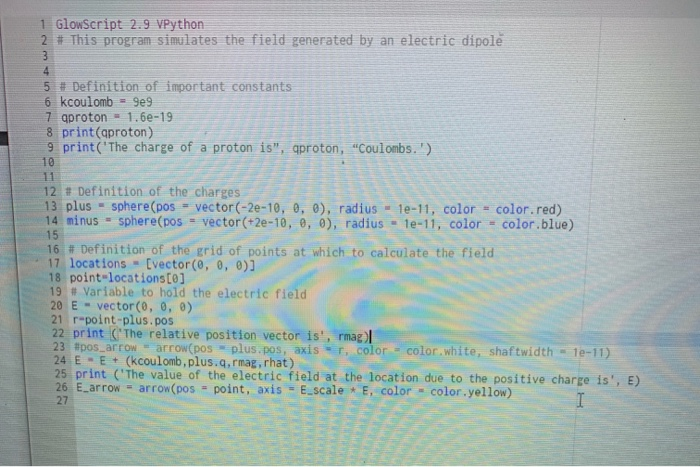
nloads/Edit%202%20Visualizing%20Electric%20Fields%20with%20VPython%20(3).pdf Now on a new line create another sphere object called 'minus'. Position it at an x-coordinate of +2e-10 with the same radius as 'plus'. Make it blue and assign it a charge of -qproton'. Part C: Calculating the electric field Before we can calculate the electric field E at a point we must define a variable that provides the locations at which we are interested in finding the field. Let's start with a single point right between the two charges. Add the following to your program: # Definition of the grid of points at which to calculate the field locations = [vector(0,0,0) point-locations[0] locations is a list or grid of points where we will eventually find the electric field. Right now, our grid only has one point, at the origin. locations[0] refers to the first and only) item in our list of locations. We use the variable point to refer to this spot. We'll come back and add more points in Part D, but for now it's easiest to calculate the electric field at just one point. Add another two lines of code: # Variable to hold the electric field E-vector(0, 0, 0) This second line initializes the electric field variable 'E' as a vector of zero length for now. We will calculate its actual value later. Now we need to find the relative position vector i between the charge and the location at which we want to find E. This is just the difference of the vectors representing the location we're interested in and the position of the source. Write a line of code given by r-point-plus.pos Lab 2 Report x Edit 2 Visualizing Electric Fields X + /Downloads/Edit%202%20Visualizing%20Electric%20Fields%20with%20VPython%20(3).pdf gumy s por ng USTUVES W EREUREYFIFRE VUE locations. We use the variable 'point' to refer to this spot. We'll come back and add more points in Part D, but for now it's easiest to calculate the electric field at just one point. Add another two lines of code: # Variable to hold the electric field E = vector(0,0,0) This second line initializes the electric field variable 'E' as a vector of zero length for now. We will calculate its actual value later. Now we need to find the relative position vector i between the charge and the location at which we want to find E. This is just the difference of the vectors representing the location we're interested in and the position of the source. Write a line of code given by r-point-plus.pos to define the position vector from the positive charge to the location we want to evaluate E. The variable 'plus.pos' is the vector that gives the position of the positive charge (Note: The variables for the actual components of the charge's position vector are 'plus.pos.x', 'plus.pos.y'. and "plus.posz'. You do not need to use these if you are just interested in the sum or difference of two PHY 151 Page 4 of 10 wnloads/Edit%202%20Visualizing%20Electric%20Fields%20with%20VPython%20(3).pdf All of this has only calculated the electric field due to the positive charge. We could just copy- paste our calculation code again below and make a few modifications to also include the negative charge, but a far more effective solution is to use a loop (which uses a particular set of code over and over again). Add a new object called "dipole' beneath the definitions of plus' and 'minus' as follows: dipole = [plus, minus This new object is called a list. The brackets define what items are bundled together into the list, in this case the two sphere objects 'plus' and 'minus'. With this list we can modify what we had previously written and place the calculations we just did inside a loop over both charges. In Python, you can quickly loop over a list and automatically assign a variable that updates to represent each item in the list element-by-element. In other words, each time the loop executes, the variable can be automatically updated to the next element in the list. The below code shows how to do this. You will need to modify the section Routine to calculate the electric field'. PHY 151 Page 6 of 10 Downloads/Edit%202%20Visualizing%20Electric%20Fields%20with%20VPython%20(3).pdf Once you have inserted the line for 'rmag', define the unit vector 'rhat using a new line of code: rhat={Insert your own expression here and then add a line that prints out that just as above. With the relative position vector to the positive charge now calculated along with its magnitude and unit vector), draw an arrow to display it on the screen: pos_arrow = arrow(pos - plus.pos, axisr, color-color.white, shaftwidth = 10-11) For this new arrow-type object "pos arrow", the position attribute is the vector locating the arrow's tail and the axis is the vector providing the arrow's orientation. You should see a white arrow representing the relative position vector show up when you run your program. Afterwards, comment out the line defining 'pos_arrow' using a # sign at the beginning of it. Finally we can calculate the value of the electric field variable 'E' at the location of interest due to the positive charge. Add a line of code that looks like E-E + Insert your own expression here) PHY 151 Page 5 of 10 ownloads/Edit%202%20Visualizing%20Electric%20Fields%20with%20VPython%20(3).pdf where inside the braces you should add a calculation using the formula for the electric field at a point due to a point charge. This expression should involve 'kcoulomb', 'plus.q'. 'rmag', and "That'. Note that the above line does not appear to make sense as a mathematical equation. This is okay because the = operator does not mean mathematical equality in Python, it just means assignment. Here we are evaluating the right-hand side first by adding the old value of the vector E' (which was (0,0,0)) to the calculated vector of the electric field due to the positive charge and storing it back in the same variable 'E'. You can add a line at this point outputting 'E': print("The value of the electric field at the location due to the positive charge is", E) Now that we've calculated 'E', we can create a new arrow to visualize it. Add the following: E_arrow = arrow(pos = point, axis =E_scale * E, color= color.yellow) Here we have defined 'E arrow' to have a tail located at the vector given by "locations and an orientation in the direction of E'. The quantity 'Escale' is an arbitrary scale factor to make the arrow comparable in size to the two spheres (otherwise the length of the arrow would be enormous because the value of 'E' is much larger as a number than the radius of the spheres). Define a new variable 'Escale' right beneath 'qproton' in your section of important constants and give it a value of 4e-22. Earrow' will be revisited later. All of this has only calculated the electric field due to the positive charge. We could just copy- paste our calculation code again below and make a few modifications to also include the negative charge, but a far more effective solution is to use a loop (which uses a particular set of code over and over again). Add a new object called 'dipole' beneath the definitions of 'plus' and 'minus'as follows: wnloads/Edit%202%20Visualizing%20Electric%20Fields%20with%20VPython%20(3).pdf All of this has only calculated the electric field due to the positive charge. We could just copy- paste our calculation code again below and make a few modifications to also include the negative charge, but a far more effective solution is to use a loop (which uses a particular set of code over and over again). Add a new object called "dipole beneath the definitions of 'plus' and 'minus' as follows: dipole = [plus, minus This new object is called a list. The brackets define what items are bundled together into the list, in this case the two sphere objects 'plus' and 'minus'. With this list we can modify what we had previously written and place the calculations we just did inside a loop over both charges. In Python, you can quickly loop over a list and automatically assign a variable that updates to represent each item in the list element-by-element. In other words, each time the loop executes, the variable can be automatically updated to the next element in the list. The below code shows how to do this. You will need to modify the section Routine to calculate the electric field'. wnloads/Edit%202%20Visualizing%20Electric%20Fields%20with%20VPython%20(3).pdf E = vector(0, 0, 0) # Routine to calculate the electric field due to both charges for charge in dipole: # This loop will run over each charge in our dipole- the plus and minus charge. Our goal is to find the electric field from each source charge and add them together. The variable "charge" will hold the source charge properties- first the plus, then the minus. When we run out of items in this list- or in this case charges, this loop will end Include here all your previous calculations of r'rmag' and 'rhar for a charge as well as the calculation for the electric field it generates. Make sure it's indented relative to the for' line above. Change any use of the word 'plus 'here to the word 'charge' so that it references the respective element of dipole, and not just 'plus !! E_arrow-arrow(pos-point, axis - Escale * E, color-color.yellow) The 'for loop is very useful in Python. In this type of loop each iteration steps through the items in a list in this case each item 'charge' in the list 'dipole") and all of the code that is indented after the colon is executed for each item in the list. Notice that 'T, 'rmag', and 'rhat are redefined when stepping to the next 'charge' in the list, but "E' just gets added to and does not get reset (we will need to reset it when are calculating the electric field at the next location). Note that after the loop is done the arrow for the electric field at that point is now plotted, this time using the total value of 'E' from all charges. Make sure you run your program to see that your output makes sense. Part D. Defining the grid of points Now that we've established how to calculate the electric field at one point, generalizing this to a mloads/Edit%202%20Visualizing%20Electric%20Fields%20with%20VPython%20(3).pdf Part D: Defining the grid of points Now that we've established how to calculate the electric field at one point, generalizing this to a calculation at many different points is easy. We simply have to create another loop over each of the elements that we are going to add to "locations'. Take all of the code that we just edited in the above section and put it within another loop: # Routine to calculate electric field for point in locations: E = vector(0,0,0) {Put the 'for' loop to calculate the electric field resulting from both charges here. Note that the 'point will be updated for every point in the locations grid, which so far is still only I spot.) This guarantees that every point in locations will be assigned an 'E_arrow'. Now we just need to add more points to "locations'. We could make 'locations' a list of vectors that we manually add PHY 151 Page 7 of 10 loads/tat%202%20visualizingo Ulectric7o20Field5%20with%20VPython%2013).pdf one by one, but this is extremely tedious and counterproductive. A better solution is to define a grid of vectors and append them to locations'. Replace the section that previously defined locations with the following code: # Definition of the grid of points at which to calculate the field locations - 0 dx = 1e-10 dy = le-10 dz=1e-10 E_arrows=0 for x in arange(-4.5e-10, 4.5e-10 + dx, dx): for y in arange(-4.5e-10, 4.5e-10 + dy, dy): for z in arange(-4.5e-10, 4.5e-10 + dz, dz): s a =vector(x, y, z) locations.append(a) Let's break this code down. We've now defined locations' as an empty list, along with increments dx', 'dy', and 'dz'. Then we define three for loops nested within each other. Each loop spans a discrete set of coordinates over 'x', 'y', and 'z', each starting at -4.5e-10 and spanning up to 4.5e- 10 in increments of le-10. (Note that the form of arange()' is 'arange(min, max, increment)', and it's a function that generates a list of equally spaced values up to but not including its second argument. So the lattice goes up to 4.5e-10, but not 4.5e-10 + le-10 - 5.5e-10). Inside the loops, each set of coordinates is assigned to a temporary vector 'a' and locations.append(a)' appends the current vector 'a' to the list "locations'. Now 'locations will contain the vectors to each point of a cubic lattice within the specified range. As a side note, the reason for choosing coordinates with half-point values is because a point located exactly on one of the charges would cause a division by zero' error in the calculation of the electric field there. loads/Edit%202%20Visualizing%20Electric%20Fields%20with%20VPython%20(3).pdf locations.append(a) Let's break this code down. We've now defined locations' as an empty list, along with increments dx', 'dy', and 'dz'. Then we define three 'for loops nested within each other. Each loop spans a discrete set of coordinates over 'X', 'y', and 'z', each starting at -4.5e-10 and spanning up to 4.5e- 10 in increments of le-10. (Note that the form of 'arange()' is 'arange(min, max, increment)', and it's a function that generates a list of equally-spaced values up to but not including its second argument. So the lattice goes up to 4.5e-10, but not 4.5e-10 + le-10 = 5.5e-10). Inside the loops, cach set of coordinates is assigned to a temporary vector 'a' and 'locations.append(a)' appends the current vector 'a' to the list "locations'. Now locations' will contain the vectors to each point of a cubic lattice within the specified range. As a side note, the reason for choosing coordinates with half-point values is because a point located exactly on one of the charges would cause a division by zero' error in the calculation of the electric field there. Since 'E arrows' has been defined as a list, our earlier definition has to be changed. It will now be rewritten from E_arrow = arrow(pos - locations, axis - E_scale * E, color-color.yellow) to E_arrows.append(arrow(pos - point, axis-E_scale E, color-color.yellow)) This line should appear after the loop that calculates E, at the same indentation level of the 'for loop that loops over the charges in the dipole. Before running your program, comment out each line within the 'for' loops of the electric field calculation that prints output. Printing to the screen is so slow that it will take your program forever to finish when it does this for each of -1000 points. The program should now show a grid of arrows representing the electric field. PHY 151 Page 8 of 10 1 GlowScript 2.9 VPython 2 # This program simulates the field generated by an electric dipole 5 # Definition of important constants 6 kcoulomb - 9e9 7 qproton = 1.6e-19 8 print(proton) 9 print('The charge of a proton is", qproton, "Coulombs.') 10 12 + Definition of the charges 13 plus - sphere(pos - vector(-2e-10, 0, 0), radius - 10-11, color - color.red) 14 minus - sphere(pos - vector(+2e-10, 0, 0), radius - 1e-11, color - color.blue) 16 # Definition of the grid of points at which to calculate the field 17 locations - [vector(0, 0, 0)] 18 point-locations[0] 19 # Variable to hold the electric field 20 E - vector(0, 0, 0) 21 r-point-plus.pos 22 print ('The relative position vector is', rmag) 23 pos_arrow-arrow(pos plus.pos, axis T, color - color white, shaftwidth - 1e-11) 24 E - E+ (kcoulomb, plus.q, rmag.rhat) 25 print ('The value of the electric field at the location due to the positive charge is', E) 26 E_arrow = arrow(pos - point, axis - , color - color.yellow) 27 nloads/Edit%202%20Visualizing%20Electric%20Fields%20with%20VPython%20(3).pdf Now on a new line create another sphere object called 'minus'. Position it at an x-coordinate of +2e-10 with the same radius as 'plus'. Make it blue and assign it a charge of -qproton'. Part C: Calculating the electric field Before we can calculate the electric field E at a point we must define a variable that provides the locations at which we are interested in finding the field. Let's start with a single point right between the two charges. Add the following to your program: # Definition of the grid of points at which to calculate the field locations = [vector(0,0,0) point-locations[0] locations is a list or grid of points where we will eventually find the electric field. Right now, our grid only has one point, at the origin. locations[0] refers to the first and only) item in our list of locations. We use the variable point to refer to this spot. We'll come back and add more points in Part D, but for now it's easiest to calculate the electric field at just one point. Add another two lines of code: # Variable to hold the electric field E-vector(0, 0, 0) This second line initializes the electric field variable 'E' as a vector of zero length for now. We will calculate its actual value later. Now we need to find the relative position vector i between the charge and the location at which we want to find E. This is just the difference of the vectors representing the location we're interested in and the position of the source. Write a line of code given by r-point-plus.pos Lab 2 Report x Edit 2 Visualizing Electric Fields X + /Downloads/Edit%202%20Visualizing%20Electric%20Fields%20with%20VPython%20(3).pdf gumy s por ng USTUVES W EREUREYFIFRE VUE locations. We use the variable 'point' to refer to this spot. We'll come back and add more points in Part D, but for now it's easiest to calculate the electric field at just one point. Add another two lines of code: # Variable to hold the electric field E = vector(0,0,0) This second line initializes the electric field variable 'E' as a vector of zero length for now. We will calculate its actual value later. Now we need to find the relative position vector i between the charge and the location at which we want to find E. This is just the difference of the vectors representing the location we're interested in and the position of the source. Write a line of code given by r-point-plus.pos to define the position vector from the positive charge to the location we want to evaluate E. The variable 'plus.pos' is the vector that gives the position of the positive charge (Note: The variables for the actual components of the charge's position vector are 'plus.pos.x', 'plus.pos.y'. and "plus.posz'. You do not need to use these if you are just interested in the sum or difference of two PHY 151 Page 4 of 10 wnloads/Edit%202%20Visualizing%20Electric%20Fields%20with%20VPython%20(3).pdf All of this has only calculated the electric field due to the positive charge. We could just copy- paste our calculation code again below and make a few modifications to also include the negative charge, but a far more effective solution is to use a loop (which uses a particular set of code over and over again). Add a new object called "dipole' beneath the definitions of plus' and 'minus' as follows: dipole = [plus, minus This new object is called a list. The brackets define what items are bundled together into the list, in this case the two sphere objects 'plus' and 'minus'. With this list we can modify what we had previously written and place the calculations we just did inside a loop over both charges. In Python, you can quickly loop over a list and automatically assign a variable that updates to represent each item in the list element-by-element. In other words, each time the loop executes, the variable can be automatically updated to the next element in the list. The below code shows how to do this. You will need to modify the section Routine to calculate the electric field'. PHY 151 Page 6 of 10 Downloads/Edit%202%20Visualizing%20Electric%20Fields%20with%20VPython%20(3).pdf Once you have inserted the line for 'rmag', define the unit vector 'rhat using a new line of code: rhat={Insert your own expression here and then add a line that prints out that just as above. With the relative position vector to the positive charge now calculated along with its magnitude and unit vector), draw an arrow to display it on the screen: pos_arrow = arrow(pos - plus.pos, axisr, color-color.white, shaftwidth = 10-11) For this new arrow-type object "pos arrow", the position attribute is the vector locating the arrow's tail and the axis is the vector providing the arrow's orientation. You should see a white arrow representing the relative position vector show up when you run your program. Afterwards, comment out the line defining 'pos_arrow' using a # sign at the beginning of it. Finally we can calculate the value of the electric field variable 'E' at the location of interest due to the positive charge. Add a line of code that looks like E-E + Insert your own expression here) PHY 151 Page 5 of 10 ownloads/Edit%202%20Visualizing%20Electric%20Fields%20with%20VPython%20(3).pdf where inside the braces you should add a calculation using the formula for the electric field at a point due to a point charge. This expression should involve 'kcoulomb', 'plus.q'. 'rmag', and "That'. Note that the above line does not appear to make sense as a mathematical equation. This is okay because the = operator does not mean mathematical equality in Python, it just means assignment. Here we are evaluating the right-hand side first by adding the old value of the vector E' (which was (0,0,0)) to the calculated vector of the electric field due to the positive charge and storing it back in the same variable 'E'. You can add a line at this point outputting 'E': print("The value of the electric field at the location due to the positive charge is", E) Now that we've calculated 'E', we can create a new arrow to visualize it. Add the following: E_arrow = arrow(pos = point, axis =E_scale * E, color= color.yellow) Here we have defined 'E arrow' to have a tail located at the vector given by "locations and an orientation in the direction of E'. The quantity 'Escale' is an arbitrary scale factor to make the arrow comparable in size to the two spheres (otherwise the length of the arrow would be enormous because the value of 'E' is much larger as a number than the radius of the spheres). Define a new variable 'Escale' right beneath 'qproton' in your section of important constants and give it a value of 4e-22. Earrow' will be revisited later. All of this has only calculated the electric field due to the positive charge. We could just copy- paste our calculation code again below and make a few modifications to also include the negative charge, but a far more effective solution is to use a loop (which uses a particular set of code over and over again). Add a new object called 'dipole' beneath the definitions of 'plus' and 'minus'as follows: wnloads/Edit%202%20Visualizing%20Electric%20Fields%20with%20VPython%20(3).pdf All of this has only calculated the electric field due to the positive charge. We could just copy- paste our calculation code again below and make a few modifications to also include the negative charge, but a far more effective solution is to use a loop (which uses a particular set of code over and over again). Add a new object called "dipole beneath the definitions of 'plus' and 'minus' as follows: dipole = [plus, minus This new object is called a list. The brackets define what items are bundled together into the list, in this case the two sphere objects 'plus' and 'minus'. With this list we can modify what we had previously written and place the calculations we just did inside a loop over both charges. In Python, you can quickly loop over a list and automatically assign a variable that updates to represent each item in the list element-by-element. In other words, each time the loop executes, the variable can be automatically updated to the next element in the list. The below code shows how to do this. You will need to modify the section Routine to calculate the electric field'. wnloads/Edit%202%20Visualizing%20Electric%20Fields%20with%20VPython%20(3).pdf E = vector(0, 0, 0) # Routine to calculate the electric field due to both charges for charge in dipole: # This loop will run over each charge in our dipole- the plus and minus charge. Our goal is to find the electric field from each source charge and add them together. The variable "charge" will hold the source charge properties- first the plus, then the minus. When we run out of items in this list- or in this case charges, this loop will end Include here all your previous calculations of r'rmag' and 'rhar for a charge as well as the calculation for the electric field it generates. Make sure it's indented relative to the for' line above. Change any use of the word 'plus 'here to the word 'charge' so that it references the respective element of dipole, and not just 'plus !! E_arrow-arrow(pos-point, axis - Escale * E, color-color.yellow) The 'for loop is very useful in Python. In this type of loop each iteration steps through the items in a list in this case each item 'charge' in the list 'dipole") and all of the code that is indented after the colon is executed for each item in the list. Notice that 'T, 'rmag', and 'rhat are redefined when stepping to the next 'charge' in the list, but "E' just gets added to and does not get reset (we will need to reset it when are calculating the electric field at the next location). Note that after the loop is done the arrow for the electric field at that point is now plotted, this time using the total value of 'E' from all charges. Make sure you run your program to see that your output makes sense. Part D. Defining the grid of points Now that we've established how to calculate the electric field at one point, generalizing this to a mloads/Edit%202%20Visualizing%20Electric%20Fields%20with%20VPython%20(3).pdf Part D: Defining the grid of points Now that we've established how to calculate the electric field at one point, generalizing this to a calculation at many different points is easy. We simply have to create another loop over each of the elements that we are going to add to "locations'. Take all of the code that we just edited in the above section and put it within another loop: # Routine to calculate electric field for point in locations: E = vector(0,0,0) {Put the 'for' loop to calculate the electric field resulting from both charges here. Note that the 'point will be updated for every point in the locations grid, which so far is still only I spot.) This guarantees that every point in locations will be assigned an 'E_arrow'. Now we just need to add more points to "locations'. We could make 'locations' a list of vectors that we manually add PHY 151 Page 7 of 10 loads/tat%202%20visualizingo Ulectric7o20Field5%20with%20VPython%2013).pdf one by one, but this is extremely tedious and counterproductive. A better solution is to define a grid of vectors and append them to locations'. Replace the section that previously defined locations with the following code: # Definition of the grid of points at which to calculate the field locations - 0 dx = 1e-10 dy = le-10 dz=1e-10 E_arrows=0 for x in arange(-4.5e-10, 4.5e-10 + dx, dx): for y in arange(-4.5e-10, 4.5e-10 + dy, dy): for z in arange(-4.5e-10, 4.5e-10 + dz, dz): s a =vector(x, y, z) locations.append(a) Let's break this code down. We've now defined locations' as an empty list, along with increments dx', 'dy', and 'dz'. Then we define three for loops nested within each other. Each loop spans a discrete set of coordinates over 'x', 'y', and 'z', each starting at -4.5e-10 and spanning up to 4.5e- 10 in increments of le-10. (Note that the form of arange()' is 'arange(min, max, increment)', and it's a function that generates a list of equally spaced values up to but not including its second argument. So the lattice goes up to 4.5e-10, but not 4.5e-10 + le-10 - 5.5e-10). Inside the loops, each set of coordinates is assigned to a temporary vector 'a' and locations.append(a)' appends the current vector 'a' to the list "locations'. Now 'locations will contain the vectors to each point of a cubic lattice within the specified range. As a side note, the reason for choosing coordinates with half-point values is because a point located exactly on one of the charges would cause a division by zero' error in the calculation of the electric field there. loads/Edit%202%20Visualizing%20Electric%20Fields%20with%20VPython%20(3).pdf locations.append(a) Let's break this code down. We've now defined locations' as an empty list, along with increments dx', 'dy', and 'dz'. Then we define three 'for loops nested within each other. Each loop spans a discrete set of coordinates over 'X', 'y', and 'z', each starting at -4.5e-10 and spanning up to 4.5e- 10 in increments of le-10. (Note that the form of 'arange()' is 'arange(min, max, increment)', and it's a function that generates a list of equally-spaced values up to but not including its second argument. So the lattice goes up to 4.5e-10, but not 4.5e-10 + le-10 = 5.5e-10). Inside the loops, cach set of coordinates is assigned to a temporary vector 'a' and 'locations.append(a)' appends the current vector 'a' to the list "locations'. Now locations' will contain the vectors to each point of a cubic lattice within the specified range. As a side note, the reason for choosing coordinates with half-point values is because a point located exactly on one of the charges would cause a division by zero' error in the calculation of the electric field there. Since 'E arrows' has been defined as a list, our earlier definition has to be changed. It will now be rewritten from E_arrow = arrow(pos - locations, axis - E_scale * E, color-color.yellow) to E_arrows.append(arrow(pos - point, axis-E_scale E, color-color.yellow)) This line should appear after the loop that calculates E, at the same indentation level of the 'for loop that loops over the charges in the dipole. Before running your program, comment out each line within the 'for' loops of the electric field calculation that prints output. Printing to the screen is so slow that it will take your program forever to finish when it does this for each of -1000 points. The program should now show a grid of arrows representing the electric field. PHY 151 Page 8 of 10 1 GlowScript 2.9 VPython 2 # This program simulates the field generated by an electric dipole 5 # Definition of important constants 6 kcoulomb - 9e9 7 qproton = 1.6e-19 8 print(proton) 9 print('The charge of a proton is", qproton, "Coulombs.') 10 12 + Definition of the charges 13 plus - sphere(pos - vector(-2e-10, 0, 0), radius - 10-11, color - color.red) 14 minus - sphere(pos - vector(+2e-10, 0, 0), radius - 1e-11, color - color.blue) 16 # Definition of the grid of points at which to calculate the field 17 locations - [vector(0, 0, 0)] 18 point-locations[0] 19 # Variable to hold the electric field 20 E - vector(0, 0, 0) 21 r-point-plus.pos 22 print ('The relative position vector is', rmag) 23 pos_arrow-arrow(pos plus.pos, axis T, color - color white, shaftwidth - 1e-11) 24 E - E+ (kcoulomb, plus.q, rmag.rhat) 25 print ('The value of the electric field at the location due to the positive charge is', E) 26 E_arrow = arrow(pos - point, axis - , color - color.yellow) 27