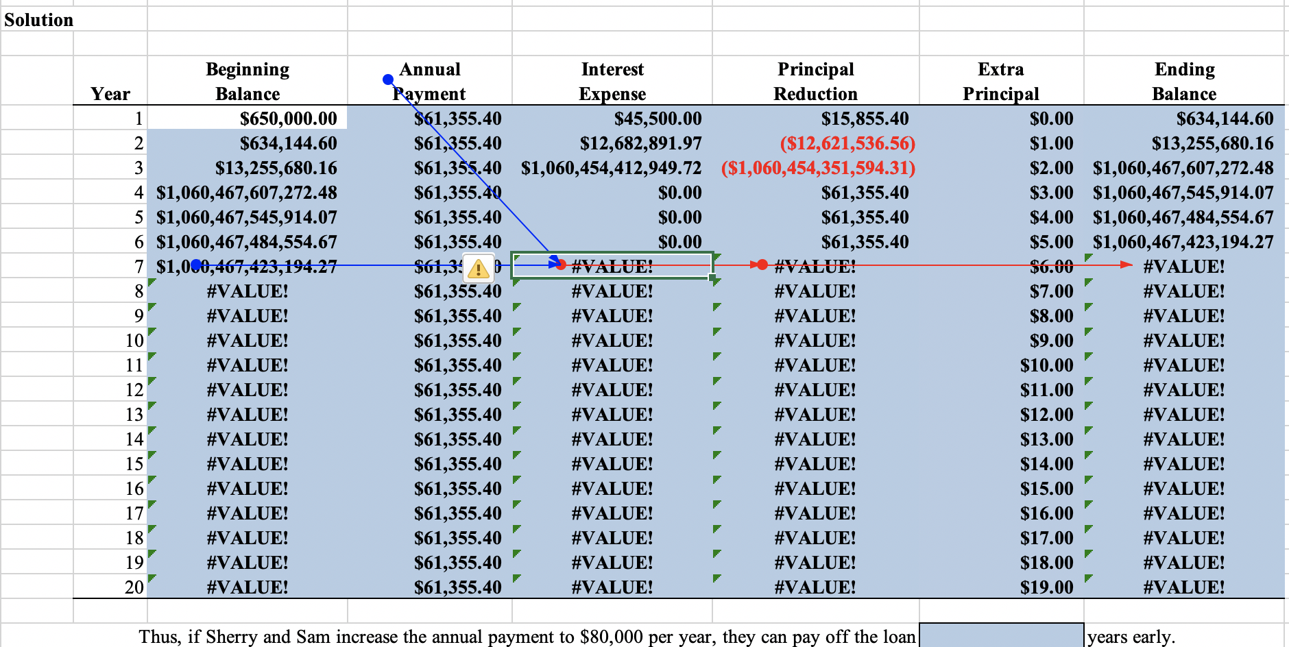
I'm having trouble with the instructions for step 9, everytime I try to drag down the values, I get an error message saying #value!, can you tell me what I'm doing wrong, thanks?

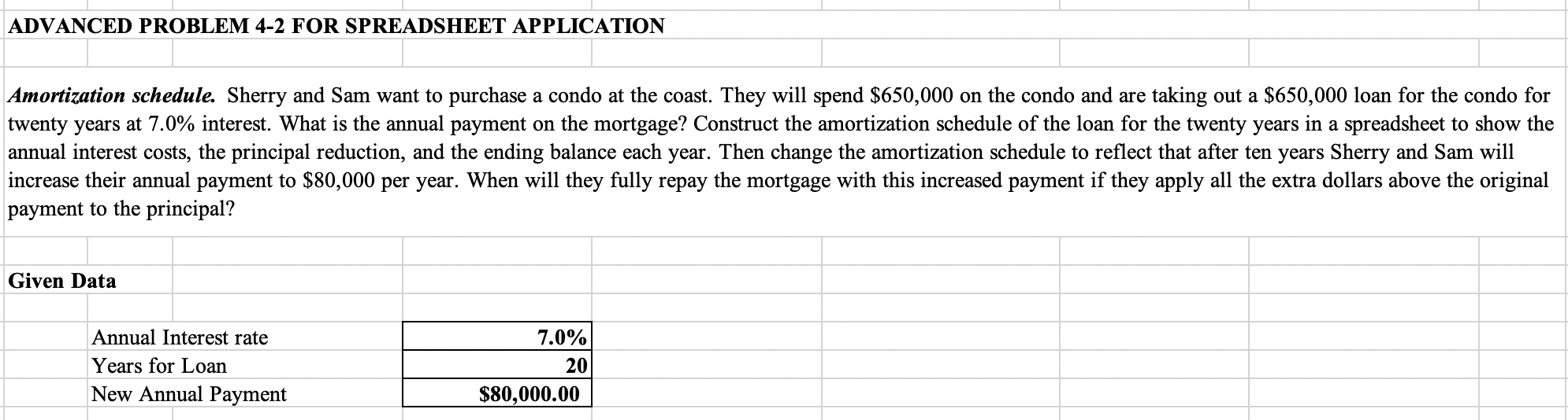
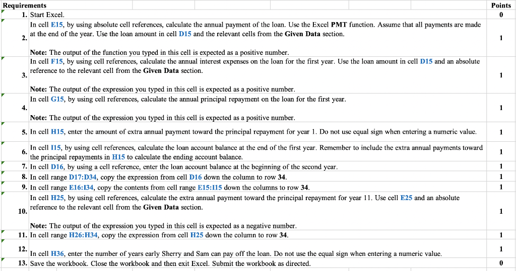
ADVANCED PROBLEM 4-2 FOR SPREADSHEET APPLICATION Amortization schedule. Sherry and Sam want to purchase a condo at the coast. They will spend $650,000 on the condo and are taking out a $650,000 loan for the condo for twenty years at 7.0% interest. What is the annual payment on the mortgage? Construct the amortization schedule of the loan for the twenty years in a spreadsheet to show the annual interest costs, the principal reduction, and the ending balance each year. Then change the amortization schedule to reflect that after ten years Sherry and Sam will increase their annual payment to $80,000 per year. When will they fully repay the mortgage with this increased payment if they apply all the extra dollars above the original payment to the principal? Given Data Annual Interest rate Years for Loan New Annual Payment 7.0% 20 $80,000.00 Solution Beginning Year Balance 1 $650,000.00 2 $634,144.60 3 $13,255,680.16 4 $1,060,467,607,272.48 5 $1,060,467,545,914.07 6 $1,060,467,484,554.67 7 $1,000,467,423,194.27 8 #VALUE! 9 #VALUE! 10 #VALUE! 11 #VALUE! 12 #VALUE! 13 #VALUE! 14 #VALUE! #VALUE! 16 #VALUE! 17 #VALUE! 18 #VALUE! 19 #VALUE! 20 #VALUE! Annual Interest Principal Payment Expense Reduction $61,355.40 $45,500.00 $15,855.40 $61,355.40 $12,682,891.97 ($12,621,536.56) $61,355.40 $1,060,454,412,949.72 ($1,060,454,351,594.31) $61,355.40 $0.00 $61,355.40 $61,355.40 $0.00 $61,355.40 $61,355.40 $0.00 $61,355.40 $61,3: o #VALUE! #VALUE! $61,355.40 #VALUE! #VALUE! $61,355.40 #VALUE! #VALUE! $61,355.40 #VALUE! #VALUE! $61,355.40 #VALUE! #VALUE! $61,355.40 #VALUE! #VALUE! $61,355.40 #VALUE! #VALUE! $61,355.40 #VALUE! #VALUE! $61,355.40 #VALUE! #VALUE! $61,355.40 #VALUE! #VALUE! $61,355.40 #VALUE! #VALUE! $61,355.40 #VALUE! #VALUE! $61,355.40 #VALUE! #VALUE! $61,355.40 #VALUE! #VALUE! Extra Ending Principal Balance $0.00 $634,144.60 $1.00 $13,255,680.16 $2.00 $1,060,467,607,272.48 $3.00 $1,060,467,545,914.07 $4.00 $1,060,467,484,554.67 $5.00 $1,060,467,423,194.27 $6.00 #VALUE! $7.00 #VALUE! $8.00 #VALUE! $9.00 #VALUE! $10.00 #VALUE! $11.00 #VALUE! $12.00 #VALUE! $13.00 #VALUE! $14.00 #VALUE! $15.00 #VALUE! $16.00 #VALUE! $17.00 #VALUE! $18.00 #VALUE! $19.00 #VALUE! 15 Thus, if Sherry and Sam increase the annual payment to $80,000 per year, they can pay off the loan years early. Points 0 Requirements 1. Start Excel. In cell E15, by using absolute cell references, calculate the annual payment of the loan. Use the Excel PMT function. Assume that all payments are made at the end of the year. Use the loan amount in cell D15 and the relevant cells from the Given Data section. 2. 1 Note: The output of the function you typed in this cell is expected as a positive number. In cell F15, by using cell references, calculate the annual interest expenses on the loan for the first year. Use the loan amount in cell D15 and an absolute reference to the relevant cell from the Given Data section. 3. 1 1 1 1 Note: The output of the expression you typed in this cell is expected as a positive number. In cell G15, by using cell references, calculate the annual principal repayment on the loan for the first year. 4. Note: The output of the expression you typed in this cell is expected as a positive number. 5. In cell H15, enter the amount of extra annual payment toward the principal repayment for year 1. Do not use equal sign when entering a numeric value. In cell 115, by using cell references, calculate the loan account balance at the end of the first year. Remember to include the extra annual payments toward 6. the principal repayments in H15 to calculate the ending account balance. 7. In cell D16, by using a cell reference, enter the loan account balance at the beginning of the second year. 8. In cell range D17:D34, copy the expression from cell D16 down the column to row 34. 9. In cell range E16:134, copy the contents from cell range E15:115 down the columns to row 34. In cell H25, by using cell references, calculate the extra annual payment toward the principal repayment for year 11. Use cell E25 and an absolute reference to the relevant cell from the Given Data section. 10. Note: The output of the expression you typed in this cell is expected as a negative number. 11. In cell range H26:H34, copy the expression from cell H25 down the column to row 34. 1 1 1 1 1 1 12. In cell H36, enter the number of years early Sherry and Sam can pay off the loan. Do not use the equal sign when entering a numeric value. 13. Save the workbook. Close the workbook and then exit Excel. Submit the workbook as directed. 0 ADVANCED PROBLEM 4-2 FOR SPREADSHEET APPLICATION Amortization schedule. Sherry and Sam want to purchase a condo at the coast. They will spend $650,000 on the condo and are taking out a $650,000 loan for the condo for twenty years at 7.0% interest. What is the annual payment on the mortgage? Construct the amortization schedule of the loan for the twenty years in a spreadsheet to show the annual interest costs, the principal reduction, and the ending balance each year. Then change the amortization schedule to reflect that after ten years Sherry and Sam will increase their annual payment to $80,000 per year. When will they fully repay the mortgage with this increased payment if they apply all the extra dollars above the original payment to the principal? Given Data Annual Interest rate Years for Loan New Annual Payment 7.0% 20 $80,000.00 Solution Beginning Year Balance 1 $650,000.00 2 $634,144.60 3 $13,255,680.16 4 $1,060,467,607,272.48 5 $1,060,467,545,914.07 6 $1,060,467,484,554.67 7 $1,000,467,423,194.27 8 #VALUE! 9 #VALUE! 10 #VALUE! 11 #VALUE! 12 #VALUE! 13 #VALUE! 14 #VALUE! #VALUE! 16 #VALUE! 17 #VALUE! 18 #VALUE! 19 #VALUE! 20 #VALUE! Annual Interest Principal Payment Expense Reduction $61,355.40 $45,500.00 $15,855.40 $61,355.40 $12,682,891.97 ($12,621,536.56) $61,355.40 $1,060,454,412,949.72 ($1,060,454,351,594.31) $61,355.40 $0.00 $61,355.40 $61,355.40 $0.00 $61,355.40 $61,355.40 $0.00 $61,355.40 $61,3: o #VALUE! #VALUE! $61,355.40 #VALUE! #VALUE! $61,355.40 #VALUE! #VALUE! $61,355.40 #VALUE! #VALUE! $61,355.40 #VALUE! #VALUE! $61,355.40 #VALUE! #VALUE! $61,355.40 #VALUE! #VALUE! $61,355.40 #VALUE! #VALUE! $61,355.40 #VALUE! #VALUE! $61,355.40 #VALUE! #VALUE! $61,355.40 #VALUE! #VALUE! $61,355.40 #VALUE! #VALUE! $61,355.40 #VALUE! #VALUE! $61,355.40 #VALUE! #VALUE! Extra Ending Principal Balance $0.00 $634,144.60 $1.00 $13,255,680.16 $2.00 $1,060,467,607,272.48 $3.00 $1,060,467,545,914.07 $4.00 $1,060,467,484,554.67 $5.00 $1,060,467,423,194.27 $6.00 #VALUE! $7.00 #VALUE! $8.00 #VALUE! $9.00 #VALUE! $10.00 #VALUE! $11.00 #VALUE! $12.00 #VALUE! $13.00 #VALUE! $14.00 #VALUE! $15.00 #VALUE! $16.00 #VALUE! $17.00 #VALUE! $18.00 #VALUE! $19.00 #VALUE! 15 Thus, if Sherry and Sam increase the annual payment to $80,000 per year, they can pay off the loan years early. Points 0 Requirements 1. Start Excel. In cell E15, by using absolute cell references, calculate the annual payment of the loan. Use the Excel PMT function. Assume that all payments are made at the end of the year. Use the loan amount in cell D15 and the relevant cells from the Given Data section. 2. 1 Note: The output of the function you typed in this cell is expected as a positive number. In cell F15, by using cell references, calculate the annual interest expenses on the loan for the first year. Use the loan amount in cell D15 and an absolute reference to the relevant cell from the Given Data section. 3. 1 1 1 1 Note: The output of the expression you typed in this cell is expected as a positive number. In cell G15, by using cell references, calculate the annual principal repayment on the loan for the first year. 4. Note: The output of the expression you typed in this cell is expected as a positive number. 5. In cell H15, enter the amount of extra annual payment toward the principal repayment for year 1. Do not use equal sign when entering a numeric value. In cell 115, by using cell references, calculate the loan account balance at the end of the first year. Remember to include the extra annual payments toward 6. the principal repayments in H15 to calculate the ending account balance. 7. In cell D16, by using a cell reference, enter the loan account balance at the beginning of the second year. 8. In cell range D17:D34, copy the expression from cell D16 down the column to row 34. 9. In cell range E16:134, copy the contents from cell range E15:115 down the columns to row 34. In cell H25, by using cell references, calculate the extra annual payment toward the principal repayment for year 11. Use cell E25 and an absolute reference to the relevant cell from the Given Data section. 10. Note: The output of the expression you typed in this cell is expected as a negative number. 11. In cell range H26:H34, copy the expression from cell H25 down the column to row 34. 1 1 1 1 1 1 12. In cell H36, enter the number of years early Sherry and Sam can pay off the loan. Do not use the equal sign when entering a numeric value. 13. Save the workbook. Close the workbook and then exit Excel. Submit the workbook as directed. 0