import numpy as np from scipy.optimize import minimize from scipy.io import loadmat from numpy.linalg import det, inv from math import sqrt, pi import scipy.io import matplotlib.pyplot as plt import pickle from sklearn.linear_model import LinearRegression from sklearn.linear_model import Ridge #%% def LinearRegressionModel(X, y, with_fit_intercept): # Inputs: # X = N x d # y = N x 1 # Output: # Linear regression model # IMPLEMENT THIS METHOD USING sklearn.linear_model.LinearRegression return clf #%% def learnOLERegression(X,y): # Inputs: # X = N x d # y = N x 1 # Output: # w = d x 1 # IMPLEMENT THIS METHOD return w #%% def testOLERegression(w,Xtest,ytest): # Inputs: # w = d x 1 # Xtest = N x d # ytest = X x 1 # Output: # mse # IMPLEMENT THIS METHOD return mse #%% def learnRidgeRegression(X,y,lambd): # Inputs: # X = N x d # y = N x 1 # lambd = ridge parameter (scalar) # Output: # w = d x 1 # IMPLEMENT THIS METHOD return w #%% def RidgeRegressionModel(X, y, alpha_value): # Inputs: # X = N x d # y = N x 1 # Output: # Linear regression model # IMPLEMENT THIS METHOD USING sklearn.linear_model.Ridge return clf #%% def mapNonLinear(x,p): # Inputs: # x - a single column vector (N x 1) # p - integer (>= 0) # Outputs: # Xd - (N x (d+1)) # IMPLEMENT THIS METHOD return Xd #%% def regressionObjVal(w, X, y, lambd): # compute squared error (scalar) and gradient of squared error with respect # to w (vector) for the given data X and y and the regularization parameter # lambda # IMPLEMENT THIS METHOD return error, error_grad #%% # Main script # Problem 1 # Input data X,y,Xtest,ytest = pickle.load(open('diabetes.pickle','rb'),encoding='latin1') # add intercept x1 = np.ones((len(X),1)) x2 = np.ones((len(Xtest),1)) X_i = np.concatenate((np.ones((X.shape[0],1)), X), axis=1) Xtest_i = np.concatenate((np.ones((Xtest.shape[0],1)), Xtest), axis=1) # Scikit package clf_without_intercept = LinearRegressionModel(X, y, False) w_lr = clf_without_intercept.coef_[0] w_lr = w_lr.reshape((len(w_lr), 1)) mle_lr = testOLERegression(w_lr,Xtest,ytest) print('Sklearn MSE without intercept '+str(mle_lr)) clf_with_intercept = LinearRegressionModel(X, y, True) w_i_lr = np.concatenate((clf_with_intercept.intercept_, clf_with_intercept.coef_[0]), axis = 0) w_i_lr = w_i_lr.reshape((len(w_i_lr), 1)) mle_i_lr = testOLERegression(w_i_lr,Xtest_i,ytest) print('Sklearn MSE with intercept '+str(mle_i_lr)) # Matrix computation w = learnOLERegression(X,y) mle = testOLERegression(w,Xtest,ytest) w_i = learnOLERegression(X_i,y) mle_i = testOLERegression(w_i,Xtest_i,ytest) print('MSE without intercept '+str(mle)) print('MSE with intercept '+str(mle_i))

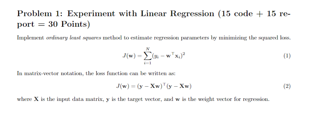
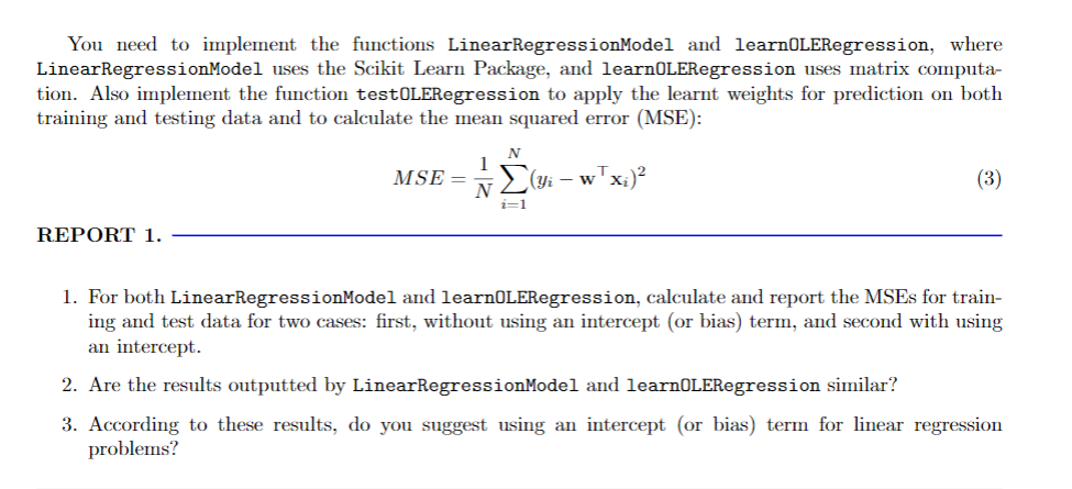
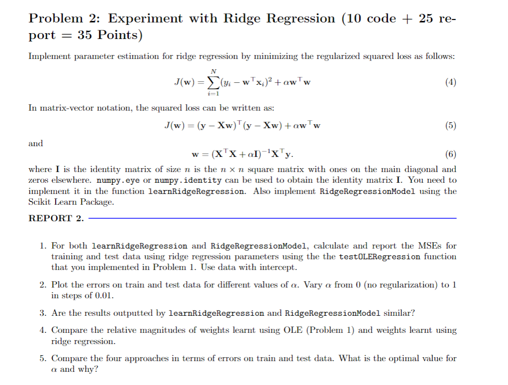
# Problem 2 k = 101 alphas = np.linspace(0, 1, num=k) i = 0 mses2_train_rr = np.zeros((k,1)) mses2_rr = np.zeros((k,1)) for alpha in alphas: clf = RidgeRegressionModel(X,y,alpha) w_l_rr = np.concatenate((clf.intercept_, clf.coef_[0]), axis = 0) w_l_rr = w_l_rr.reshape((len(w_l_rr), 1)) mses2_train_rr[i] = testOLERegression(w_l_rr,X_i,y) mses2_rr[i] = testOLERegression(w_l_rr,Xtest_i,ytest) i = i + 1 fig = plt.figure(figsize=[12,6]) plt.subplot(1, 2, 1) plt.plot(alphas,mses2_train_rr) plt.title('Sklearn MSE for Train Data') plt.subplot(1, 2, 2) plt.plot(alphas,mses2_rr) plt.title('Sklearn MSE for Test Data') i = 0 mses2_train = np.zeros((k,1)) mses2 = np.zeros((k,1)) for alpha in alphas: w_l = learnRidgeRegression(X_i,y,alpha) mses2_train[i] = testOLERegression(w_l,X_i,y) mses2[i] = testOLERegression(w_l,Xtest_i,ytest) i = i + 1 fig = plt.figure(figsize=[12,6]) plt.subplot(1, 2, 1) plt.plot(alphas,mses2_train) plt.title('MSE for Train Data') plt.subplot(1, 2, 2) plt.plot(alphas,mses2) plt.title('MSE for Test Data') #%% # Problem 3 pmax = 7 #alpha_opt = 0 # REPLACE THIS WITH alpha_opt estimated from Problem 2 alpha_opt = alphas[np.argmin(mses2)] mses3_train = np.zeros((pmax,2)) mses3 = np.zeros((pmax,2)) for p in range(pmax): Xd = mapNonLinear(X[:,2],p) Xdtest = mapNonLinear(Xtest[:,2],p) w_d1 = learnRidgeRegression(Xd,y,0) mses3_train[p,0] = testOLERegression(w_d1,Xd,y) mses3[p,0] = testOLERegression(w_d1,Xdtest,ytest) w_d2 = learnRidgeRegression(Xd,y,lambda_opt) mses3_train[p,1] = testOLERegression(w_d2,Xd,y) mses3[p,1] = testOLERegression(w_d2,Xdtest,ytest) fig = plt.figure(figsize=[12,6]) plt.subplot(1, 2, 1) plt.plot(range(pmax),mses4_train) plt.title('MSE for Train Data') plt.legend(('No Regularization','Regularization')) plt.subplot(1, 2, 2) plt.plot(range(pmax),mses4) plt.title('MSE for Test Data') plt.legend(('No Regularization','Regularization')) #%% # Problem 5 fig = plt.figure(figsize=[10,8]) k = 101 lambdas = np.linspace(0, 1, num=k) i = 0 mses5_train = np.zeros((k,1)) mses5 = np.zeros((k,1)) opts = {'maxiter' : 20} # Preferred value. w_init = np.ones((X_i.shape[1],1)) for lambd in lambdas: args = (X_i, y, lambd) w_l = minimize(regressionObjVal, w_init, jac=True, args=args,method='CG', options=opts) w_l = np.transpose(np.array(w_l.x)) w_l = np.reshape(w_l,[len(w_l),1]) mses5_train[i] = testOLERegression(w_l,X_i,y) mses5[i] = testOLERegression(w_l,Xtest_i,ytest) i = i + 1 fig = plt.figure(figsize=[12,6]) plt.subplot(1, 2, 1) plt.plot(lambdas,mses5_train) plt.plot(lambdas,mses2_train) plt.title('MSE for Train Data') plt.legend(['Using scipy.minimize','Direct minimization']) plt.subplot(1, 2, 2) plt.plot(lambdas,mses5) plt.plot(lambdas,mses2) plt.title('MSE for Test Data') plt.legend(['Using scipy.minimize','Direct minimization'])

Data Set A medical data set is provided in the file "diabetes.pickle along with the target assignment. The input variables correspond to measurements (physical, physiological, and blood related) for a given patient and the target variable corresponds to the level of diabetic condition in the patient. It contains: Xtrain (242 x 64) and ytrain (242 x 1) for training. Xtest (200 x 64) and ytost (200 x 1) for testing. Problem 1: Experiment with Linear Regression (15 code + 15 re- port = 30 Points) Implement ordinary least squares method to estimate regression parameters by minimizing the squared loss. J(w) = x)2 (yi - w i=1 In matrix-vector notation, the loss function can be written as: J(w) = (y - Xw)(y - Xw) where X is the input data matrix, y is the target vector, and w is the weight vector for regression. You need to implement the functions LinearRegressionModel and learnOLERegression, where LinearRegressionModel uses the Scikit Learn Package, and learnOLERegression uses matrix computa- tion. Also implement the function testOLERegression to apply the learnt weights for prediction on both training and testing data and to calculate the mean squared error (MSE): (Yi - wTxi2 (3) REPORT 1. 1. For both LinearRegressionModel and learnOLERegression, calculate and report the MSEs for train- ing and test data for two cases: first, without using an intercept (or bias) term, and second with using an intercept. 2. Are the results outputted by LinearRegressionModel and learnOLERegression similar? for linear regression 3. According to these results, do you suggest using an intercept (or bias) term problems? Problem 2: Experiment with Ridge Regression (10 code + 25 re- port = 35 Points) Implement parameter estimation for ridge regression by minimizing the regularized squared loss as follows: N J(w) = (yi - wTx;)+aww 2=1 In matrix-vector notation, the squared loss can be written as: J(w) = (y - Xw)'(y - Xw) +aw'w (6) and w=(xx+al)-'xty. where I is the identity matrix of size n is the n x n square matrix with ones on the main diagonal and zeros elsewhere. numpy.eye or numpy.identity can be used to obtain the identity matrix I. You need to implement it in the function learnRidgeRegression. Also implement RidgeRegressionModel using the Scikit Learn Package. REPORT 2. ILLIUILI A. 1. For both learnRidgeRegression and RidgeRegressionModel, calculate and report the MSEs for training and test data using ridge regression parameters using the the test OLERegression function that you implemented in Problem 1. Use data with intercept. 2. Plot the errors on train and test data for different values of a. Vary a from 0 (no regularization) to 1 in steps of 0.01. 3. Are the results outputted by learnRidgeRegression and RidgeRegressionModel similar? 4. Compare the relative magnitudes of weights learnt using OLE (Problem 1) and weights learnt using ridge regression. 5. Compare the four approaches in terms of errors on train and test data. What is the optimal value for a and why? Problem 3: Non-linear Regression (10 code + 15 report = 25 Points) In this problem we will investigate the impact of using higher order polynomials for the input features. For this problem use the third variable as the only input variable: x-train = x-train: ,2] x-test = x-test (:, 2] Implement the function mapNonLinear which converts a single attribute x into a vector of p attributes, 1, 1, 2,..., I. REPORT 3 Using the a = 0 and the optimal value of a found in Problem 2, train ridge regression weights using the non-linear mapping of the data. Vary p from 0 to 6. Note that p=0 means using a horizontal line as the regression line, p=1 is the same as linear ridge regression. 1. Compute the errors on train and test data for different p's. Compare the results for both values of a. 2. What is the optimal value of p in terms of test crror in cach setting? 3. Plot the curve for the optimal value of p for both values of a and compare. Problem 4: Interpreting Results (0 code + 10 report = 10 points) Using the results obtained for the first 3 problems, make final recommendations for anyone using regression for predicting diabetes level using the input features. REPORT 4. Compare the various approaches in terms of training and testing error. What metric should be used to choose the best setting? Bonus Problem 5: Using Gradient Descent for Ridge Regression Learning (15 code + 5 report = 20 Points) As discussed in class, regression parameters can be calculated directly using analytical expressions (as in Problem 1 and 2). To avoid computation of (XTX)-1, another option is to use gradient descent to minimize the loss function (or to maximize the log-likelihood) function. In this problem, you have to implement the gradient descent procedure for estimating the weights w. You need to use the minimize function (from the scipy library) which is same as the minimizer that you used for first assignment. You need to implement a function regressionObjVal to compute the regularized squared error (See (4)) and its gradient with respect to w. In the main script, this objective function will be used within the minimizer. REPORT 5. Plot the errors on train and test data obtained by using the gradient descent based learning by varying the regularization parameter a. Compare with the results obtained in Problem 2. Is it better than the first three approaches? Why? Data Set A medical data set is provided in the file "diabetes.pickle along with the target assignment. The input variables correspond to measurements (physical, physiological, and blood related) for a given patient and the target variable corresponds to the level of diabetic condition in the patient. It contains: Xtrain (242 x 64) and ytrain (242 x 1) for training. Xtest (200 x 64) and ytost (200 x 1) for testing. Problem 1: Experiment with Linear Regression (15 code + 15 re- port = 30 Points) Implement ordinary least squares method to estimate regression parameters by minimizing the squared loss. J(w) = x)2 (yi - w i=1 In matrix-vector notation, the loss function can be written as: J(w) = (y - Xw)(y - Xw) where X is the input data matrix, y is the target vector, and w is the weight vector for regression. You need to implement the functions LinearRegressionModel and learnOLERegression, where LinearRegressionModel uses the Scikit Learn Package, and learnOLERegression uses matrix computa- tion. Also implement the function testOLERegression to apply the learnt weights for prediction on both training and testing data and to calculate the mean squared error (MSE): (Yi - wTxi2 (3) REPORT 1. 1. For both LinearRegressionModel and learnOLERegression, calculate and report the MSEs for train- ing and test data for two cases: first, without using an intercept (or bias) term, and second with using an intercept. 2. Are the results outputted by LinearRegressionModel and learnOLERegression similar? for linear regression 3. According to these results, do you suggest using an intercept (or bias) term problems? Problem 2: Experiment with Ridge Regression (10 code + 25 re- port = 35 Points) Implement parameter estimation for ridge regression by minimizing the regularized squared loss as follows: N J(w) = (yi - wTx;)+aww 2=1 In matrix-vector notation, the squared loss can be written as: J(w) = (y - Xw)'(y - Xw) +aw'w (6) and w=(xx+al)-'xty. where I is the identity matrix of size n is the n x n square matrix with ones on the main diagonal and zeros elsewhere. numpy.eye or numpy.identity can be used to obtain the identity matrix I. You need to implement it in the function learnRidgeRegression. Also implement RidgeRegressionModel using the Scikit Learn Package. REPORT 2. ILLIUILI A. 1. For both learnRidgeRegression and RidgeRegressionModel, calculate and report the MSEs for training and test data using ridge regression parameters using the the test OLERegression function that you implemented in Problem 1. Use data with intercept. 2. Plot the errors on train and test data for different values of a. Vary a from 0 (no regularization) to 1 in steps of 0.01. 3. Are the results outputted by learnRidgeRegression and RidgeRegressionModel similar? 4. Compare the relative magnitudes of weights learnt using OLE (Problem 1) and weights learnt using ridge regression. 5. Compare the four approaches in terms of errors on train and test data. What is the optimal value for a and why? Problem 3: Non-linear Regression (10 code + 15 report = 25 Points) In this problem we will investigate the impact of using higher order polynomials for the input features. For this problem use the third variable as the only input variable: x-train = x-train: ,2] x-test = x-test (:, 2] Implement the function mapNonLinear which converts a single attribute x into a vector of p attributes, 1, 1, 2,..., I. REPORT 3 Using the a = 0 and the optimal value of a found in Problem 2, train ridge regression weights using the non-linear mapping of the data. Vary p from 0 to 6. Note that p=0 means using a horizontal line as the regression line, p=1 is the same as linear ridge regression. 1. Compute the errors on train and test data for different p's. Compare the results for both values of a. 2. What is the optimal value of p in terms of test crror in cach setting? 3. Plot the curve for the optimal value of p for both values of a and compare. Problem 4: Interpreting Results (0 code + 10 report = 10 points) Using the results obtained for the first 3 problems, make final recommendations for anyone using regression for predicting diabetes level using the input features. REPORT 4. Compare the various approaches in terms of training and testing error. What metric should be used to choose the best setting? Bonus Problem 5: Using Gradient Descent for Ridge Regression Learning (15 code + 5 report = 20 Points) As discussed in class, regression parameters can be calculated directly using analytical expressions (as in Problem 1 and 2). To avoid computation of (XTX)-1, another option is to use gradient descent to minimize the loss function (or to maximize the log-likelihood) function. In this problem, you have to implement the gradient descent procedure for estimating the weights w. You need to use the minimize function (from the scipy library) which is same as the minimizer that you used for first assignment. You need to implement a function regressionObjVal to compute the regularized squared error (See (4)) and its gradient with respect to w. In the main script, this objective function will be used within the minimizer. REPORT 5. Plot the errors on train and test data obtained by using the gradient descent based learning by varying the regularization parameter a. Compare with the results obtained in Problem 2. Is it better than the first three approaches? Why