

Answered step by step
Verified Expert Solution
Question
1 Approved Answer
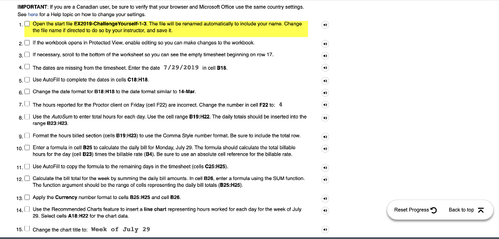
IMPORTANT: If you are a Canadian user, be sure to verify that your browser and Microsoft Office use the same country settings. See here for

Step by Step Solution
There are 3 Steps involved in it
Step: 1

Get Instant Access to Expert-Tailored Solutions
See step-by-step solutions with expert insights and AI powered tools for academic success
Step: 2

Step: 3
Ace Your Homework with AI
Get the answers you need in no time with our AI-driven, step-by-step assistance
Get Started
Oracle Autonomous Database In Enterprise Architecture
Authors: Bal Mukund Sharma, Krishnakumar KM, Rashmi Panda
1st Edition
1801072248, 978-1801072243