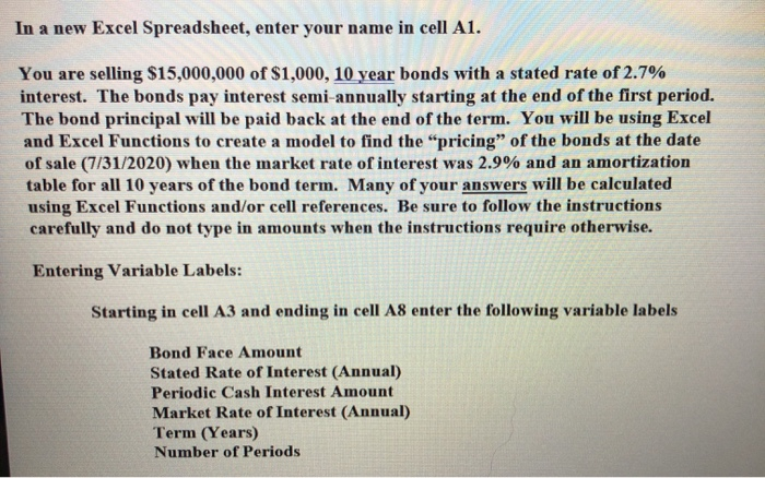
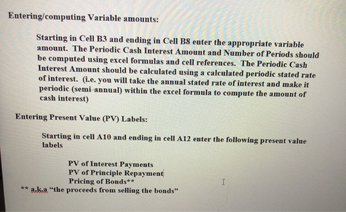
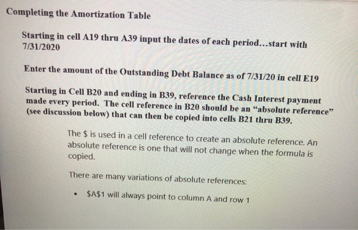
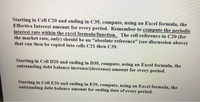
In a new Excel Spreadsheet, enter your name in cell A1. You are selling $15,000,000 of $1,000, 10 year bonds with a stated rate of 2.7% interest. The bonds pay interest semi-annually starting at the end of the first period. The bond principal will be paid back at the end of the term. You will be using Excel and Excel Functions to create a model to find the "pricing" of the bonds at the date of sale (7/31/2020) when the market rate of interest was 2.9% and an amortization table for all 10 years of the bond term. Many of your answers will be calculated using Excel Functions and/or cell references. Be sure to follow the instructions carefully and do not type in amounts when the instructions require otherwise. Entering Variable Labels: Starting in cell A3 and ending in cell A8 enter the following variable labels Bond Face Amount Stated Rate of Interest (Annual) Periodic Cash Interest Amount Market Rate of Interest (Annual) Term (Years) Number of Periods Entering/computing Variable amounts: Starting in Cell B3 and ending in Cell B8 enter the appropriate variable amount. The Periodic Cash Interest Amount and Number of Periods should be computed using excel formulas and cell references. The Periodic Cash Interest Amount should be calculated using a calculated periodic stated rate of interest. (i.e. you will take the annual stated rate of interest and make it periodic (semi-annual) within the excel formula to compute the amount of cash interest) Entering Present Value (PV) Labels: Starting in cell A10 and ending in cell A12 enter the following present value labels PV of Interest Payments PV of Principle Repayment Pricing of Bonds** a.k.a "the proceeds from selling the bonds" I Compute the Present Value amounts and the total Pricing of the Bonds on 7/31/20: Using the PV function, determine the present value of all bond cash interest payments in cell B10 Using the PV function, determine the present value of the bond principle repayment in cell B11 Using an Excel formula, determine the total pricing of the bonds in cell B12 Completing the Amortization Table Starting in cell A19 thru A39 input the dates of each period...start with 7/31/2020 Enter the amount of the Outstanding Debt Balance as of 7/31/20 in cell E19 Starting in Cell B20 and ending in B39, reference the Cash Interest payment made every period. The cell reference in B20 should be an "absolute reference" (see discussion below) that can then be copied into cells B21 thru B39. The $ is used in a cell reference to create an absolute reference. An absolute reference is one that will not change when the formula is copied There are many variations of absolute references: . $A$1 will always point to column A and row 1 Starting in Cell C20 and ending in C39, compute, using an Excel formula, the Effective Interest amount for every period. Remember to compute the periodic interest rate within the excel formula/function. The cell reference in C20 (for the market rate, only) should be an "absolute reference" (see discussion above) that can then be copied into cells C21 thru C39. Starting in Cell D20 and ending in D39, compute, using an Excel formula, the outstanding debt balance increase/(decrease) amount for every period. Starting in Cell E20 and ending in E39, compute, using an Excel formula, the outstanding debt balance amount for ending date of every period. In a new Excel Spreadsheet, enter your name in cell A1. You are selling $15,000,000 of $1,000, 10 year bonds with a stated rate of 2.7% interest. The bonds pay interest semi-annually starting at the end of the first period. The bond principal will be paid back at the end of the term. You will be using Excel and Excel Functions to create a model to find the "pricing" of the bonds at the date of sale (7/31/2020) when the market rate of interest was 2.9% and an amortization table for all 10 years of the bond term. Many of your answers will be calculated using Excel Functions and/or cell references. Be sure to follow the instructions carefully and do not type in amounts when the instructions require otherwise. Entering Variable Labels: Starting in cell A3 and ending in cell A8 enter the following variable labels Bond Face Amount Stated Rate of Interest (Annual) Periodic Cash Interest Amount Market Rate of Interest (Annual) Term (Years) Number of Periods Entering/computing Variable amounts: Starting in Cell B3 and ending in Cell B8 enter the appropriate variable amount. The Periodic Cash Interest Amount and Number of Periods should be computed using excel formulas and cell references. The Periodic Cash Interest Amount should be calculated using a calculated periodic stated rate of interest. (i.e. you will take the annual stated rate of interest and make it periodic (semi-annual) within the excel formula to compute the amount of cash interest) Entering Present Value (PV) Labels: Starting in cell A10 and ending in cell A12 enter the following present value labels PV of Interest Payments PV of Principle Repayment Pricing of Bonds** a.k.a "the proceeds from selling the bonds" I Compute the Present Value amounts and the total Pricing of the Bonds on 7/31/20: Using the PV function, determine the present value of all bond cash interest payments in cell B10 Using the PV function, determine the present value of the bond principle repayment in cell B11 Using an Excel formula, determine the total pricing of the bonds in cell B12 Completing the Amortization Table Starting in cell A19 thru A39 input the dates of each period...start with 7/31/2020 Enter the amount of the Outstanding Debt Balance as of 7/31/20 in cell E19 Starting in Cell B20 and ending in B39, reference the Cash Interest payment made every period. The cell reference in B20 should be an "absolute reference" (see discussion below) that can then be copied into cells B21 thru B39. The $ is used in a cell reference to create an absolute reference. An absolute reference is one that will not change when the formula is copied There are many variations of absolute references: . $A$1 will always point to column A and row 1 Starting in Cell C20 and ending in C39, compute, using an Excel formula, the Effective Interest amount for every period. Remember to compute the periodic interest rate within the excel formula/function. The cell reference in C20 (for the market rate, only) should be an "absolute reference" (see discussion above) that can then be copied into cells C21 thru C39. Starting in Cell D20 and ending in D39, compute, using an Excel formula, the outstanding debt balance increase/(decrease) amount for every period. Starting in Cell E20 and ending in E39, compute, using an Excel formula, the outstanding debt balance amount for ending date of every period


