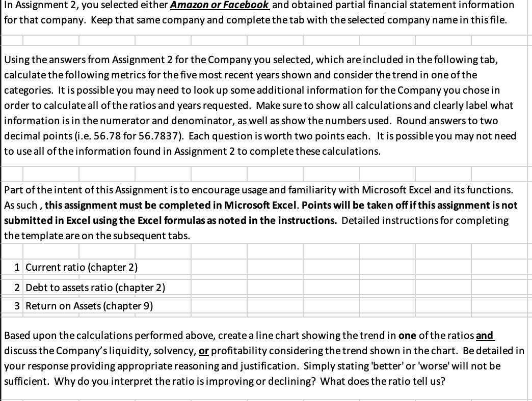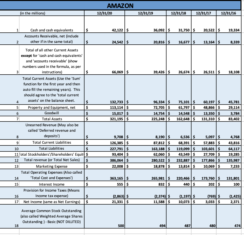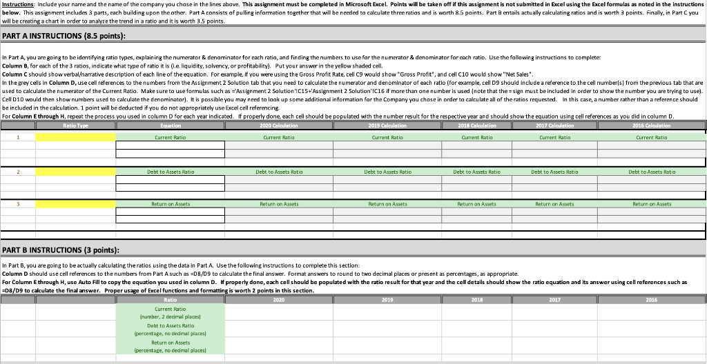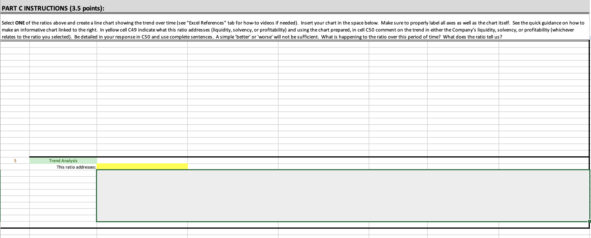
In Assignment 2, you selected either Amazon or Facebook and obtained partial financial statement information for that company. Keep that same company and complete the tab with the selected company name in this file. Using the answers from Assignment 2 for the Company you selected, which are included in the following tab, calculate the following metrics for the five most recent years shown and consider the trend in one of the categories. It is possible you may need to look up some additional information for the Company you chose in order to calculate all of the ratios and years requested. Make sure to show all calculations and clearly label what information is in the numerator and denominator, as well as show the numbers used. Round answers to two decimal points (i.e. 56.78 for 56.7837). Each question is worth two points each. It is possible you may not need to use all of the information found in Assignment 2 to complete these calculations. Part of the intent of this Assignment is to encourage usage and familiarity with Microsoft Excel and its functions. As such, this assignment must be completed in Microsoft Excel. Points will be taken off if this assignment is not submitted in Excel using the Excel formulas as noted in the instructions. Detailed instructions for completing the template are on the subsequent tabs. 1 Current ratio (chapter 2) 2 Debt to assets ratio (chapter 2) 3 Return on Assets (chapter 9) Based upon the calculations performed above, create a line chart showing the trend in one of the ratios and discuss the Company's liquidity, solvency, or profitability considering the trend shown in the chart. Be detailed in your response providing appropriate reasoning and justification. Simply stating 'better' or 'worse' will not be sufficient. Why do you interpret the ratio is improving or declining? What does the ratio tell us? AMAZON 12/31/20 (in the millions) 12/31/19 12/31/18 12/31/17 12/31/16 1 $ 42,122 $ 36,092 $ 31,750 $ 20,522 $ 19,334 Cash and cash equivalents Accounts Receivable, net (include other if in the same total) 2 $ 24,542 $ 20,816 $ 16,677 $ 13,164 $ 8,339 66,069 $ 39,426 $ 26,674 $ 26,511$ 18,108 132,733 $ 113,114$ 15,017$ 321,195 $ 96,334 $ 72,705$ 14,754 $ 225,248$ 75,101 $ 61,797 $ 14,548$ 162,648$ 60,197 $ 48,866 $ 13,350 $ 131,310$ 45,781 29,114 3,784 83,402 Total of all other Current Assets except for 'cash and cash equivalents' and 'accounts receivable' (show numbers used in the formula, as per 3 instructions) $ Total Current Assets (Use the 'Sum' function for the first year and then auto fill the remaining years). This should agree to the 'total current 4 assets' on the balance sheet. $ 5 Property and Equipment, net $ 6 Goodwill $ 7 Total Assets $ Unearned Revenue (May also be called 'Deferred revenue and 8 deposits") $ 9 Total Current Liabilities $ 10 Total Liabilities $ 11 Total Stockholders'/Shareholders' Equity $ 12 Total revenue (or Total Net Sales) $ 13 Marketing Expense $ Total Operating Expenses (Also called 14 'Total Cost and Expenses') $ 15 Interest Income $ Provision for Income Taxes (Means 16 Income tax expense) $ 17 Net Income (same as Net Earnings) $ 9,708$ 126,385$ 227,791 $ 93,404 $ 386,064 $ 22,008 $ 8,190 $ 87,812 $ 163,188 $ 62,060 $ 280,522 $ 18,878 $ 6,536 $ 68,391 $ 119,099 $ 43,549 $ 232,887 $ 13,814 $ 5,097 $ 57,883 $ 103,601$ 27,709 $ 177,866 $ 10,069 $ 4,768 43,816 64,117 19,285 135,987 7,233 363,165$ 555$ 265,981 $ 832 $ 220,466 $ 440$ 173,760$ 202 $ 131,801 100 (2,863) $ 21,331 $ (2,374) $ 11,588 $ (1,197) $ 10,073 $ (769) $ 3,033 $ (1,425) 2,371 Average Common Stock Outstanding (also called Weighted Average Shares Outstanding ) - Basic (NOT DILUTED) 18 500 494 487 480 4741 Instructions: Include your name and the name of the company you chose in the lines above. This assignment must be completed in Microsoft Excel. Points will be taken off if this assignment is not submitted in Excel using the Excel formulas as noted in the instructions below. This assignment includes 3 parts, each building upon the other. Part A consists of pulling information together that will be needed to calculate three ratios and is worth 8.5 points. Part entails actually calculating ratios and is worth 3 points. Finally, in Part you will be creating a chart in order to analyze the trend in a ratio and it is worth 3.5 points PART A INSTRUCTIONS (8.5 points): In Part A, you are going to be identifying ratio types, explaining the numerator & denominator for each ratio, and finding the numbers to use for the numerator & denominator for each ratio. Use the following instructions to complete Column B, for each of the 3 ratios, indicate what type of ratio it is (ie liquidity, solvency, or profitability). Put your answer in the yellow shaded cell. Column C should show verbal narrative description of each line of the equation. For example, if you were using the Gross Profit Rate, cell C9 would show "Gross Profit", and cell C10 would show "Net Sales'. In the grey cells in Column D, use cell references to the numbers from the Assignment Solution tab that you need to calculate the numerator and denominator of each ratio (for example, cell D9 should include a reference to the cell number(s) from the previous tab that are used to calculate the numerator of the Current Ratio. Make sure to use formulas such as ='Assignment 2 Solution'!C15+'Assignment Solution'!C16 if more than one number is used (note that the=sign must be included in order to show the number you are trying to use). Cell D10 would then show numbers used to calculate the denominator). It is possible you may need to look up some additional information for the Company you chose in order to calculate all of the ratios requested. In this case, a number rather than a reference should be included in the calculation. 1 point will be deducted if you do not appropriately use Excel cell referencing For Column Ethrough H, repeat the process you used in column D for each year indicated. If properly done, each cell should be populated with the number result for the respective year and should show the equation using cell references as you did in column D. Ratio Type Equation 2020 Calculation 2019 Calculation 2018 Calculation 2017 Calculation 2016 Calculation 1 Current Ratio Current Ratio Current Ratio Current Ratio Current Ratio Current Ratio 2 Debt to Assets Ratio Debt to Assets Ratio Debt to Assets Ratio Debt to Assets Ratio Debt to Assets Ratio Debt to Assets Ratio 3 Return on Assets Return on Assets Return on Assets Return on Assets Return on Assets Return on Assets PART B INSTRUCTIONS (3 points): In Part B, you are going to be actually calculating the ratios using the data in Part A Use the following instructions to complete this section: Column D should use cell references to the numbers from Part A such as EDB/D9 to calculate the final answer. Format answers to round to two decimal places or present as percentages, as appropriate. For Column Ethrough H, use Auto Fill to copy the equation you used in column D. of properly done, cach cell should be populated with the ratio result for that year and the cell details should show the ratio equation and its answer using cell references such as =D8/D9 to calculate the final answer. Proper usage of Excel functions and formatting is worth 2 points in this section. Ratio 2020 2019 2018 2017 2016 Current Ratio (number, 2 dedmal places Debt to Assets Ratio (percentage, no decimal places Return on Assets Ipercentage, no decimal places PART C INSTRUCTIONS (3.5 points): Select ONE of the ratios above and create a line chart showing the trend over time (see "Excel References" tab for how-to videos if needed). Insert your chart in the space below. Make sure to properly label all axes as well as the chart itself. See the quick guidance on how to make an informative chart linked to the right. In yellow cell 049 indicate what this ratio addresses (liquidity, solvency, or profitability) and using the chart prepared, in cell C50 comment on the trend in either the Company's liquidity, solvency, or profitability (whichever relates to the ratio you selected). Be detailed in your response in c50 and use complete sentences. A simple 'better' or 'worse will not be sufficient. What is happening to the ratio over this period of time? What does the ratio tell us? 5 Trend Analysis This ratio addresses: In Assignment 2, you selected either Amazon or Facebook and obtained partial financial statement information for that company. Keep that same company and complete the tab with the selected company name in this file. Using the answers from Assignment 2 for the Company you selected, which are included in the following tab, calculate the following metrics for the five most recent years shown and consider the trend in one of the categories. It is possible you may need to look up some additional information for the Company you chose in order to calculate all of the ratios and years requested. Make sure to show all calculations and clearly label what information is in the numerator and denominator, as well as show the numbers used. Round answers to two decimal points (i.e. 56.78 for 56.7837). Each question is worth two points each. It is possible you may not need to use all of the information found in Assignment 2 to complete these calculations. Part of the intent of this Assignment is to encourage usage and familiarity with Microsoft Excel and its functions. As such, this assignment must be completed in Microsoft Excel. Points will be taken off if this assignment is not submitted in Excel using the Excel formulas as noted in the instructions. Detailed instructions for completing the template are on the subsequent tabs. 1 Current ratio (chapter 2) 2 Debt to assets ratio (chapter 2) 3 Return on Assets (chapter 9) Based upon the calculations performed above, create a line chart showing the trend in one of the ratios and discuss the Company's liquidity, solvency, or profitability considering the trend shown in the chart. Be detailed in your response providing appropriate reasoning and justification. Simply stating 'better' or 'worse' will not be sufficient. Why do you interpret the ratio is improving or declining? What does the ratio tell us? AMAZON 12/31/20 (in the millions) 12/31/19 12/31/18 12/31/17 12/31/16 1 $ 42,122 $ 36,092 $ 31,750 $ 20,522 $ 19,334 Cash and cash equivalents Accounts Receivable, net (include other if in the same total) 2 $ 24,542 $ 20,816 $ 16,677 $ 13,164 $ 8,339 66,069 $ 39,426 $ 26,674 $ 26,511$ 18,108 132,733 $ 113,114$ 15,017$ 321,195 $ 96,334 $ 72,705$ 14,754 $ 225,248$ 75,101 $ 61,797 $ 14,548$ 162,648$ 60,197 $ 48,866 $ 13,350 $ 131,310$ 45,781 29,114 3,784 83,402 Total of all other Current Assets except for 'cash and cash equivalents' and 'accounts receivable' (show numbers used in the formula, as per 3 instructions) $ Total Current Assets (Use the 'Sum' function for the first year and then auto fill the remaining years). This should agree to the 'total current 4 assets' on the balance sheet. $ 5 Property and Equipment, net $ 6 Goodwill $ 7 Total Assets $ Unearned Revenue (May also be called 'Deferred revenue and 8 deposits") $ 9 Total Current Liabilities $ 10 Total Liabilities $ 11 Total Stockholders'/Shareholders' Equity $ 12 Total revenue (or Total Net Sales) $ 13 Marketing Expense $ Total Operating Expenses (Also called 14 'Total Cost and Expenses') $ 15 Interest Income $ Provision for Income Taxes (Means 16 Income tax expense) $ 17 Net Income (same as Net Earnings) $ 9,708$ 126,385$ 227,791 $ 93,404 $ 386,064 $ 22,008 $ 8,190 $ 87,812 $ 163,188 $ 62,060 $ 280,522 $ 18,878 $ 6,536 $ 68,391 $ 119,099 $ 43,549 $ 232,887 $ 13,814 $ 5,097 $ 57,883 $ 103,601$ 27,709 $ 177,866 $ 10,069 $ 4,768 43,816 64,117 19,285 135,987 7,233 363,165$ 555$ 265,981 $ 832 $ 220,466 $ 440$ 173,760$ 202 $ 131,801 100 (2,863) $ 21,331 $ (2,374) $ 11,588 $ (1,197) $ 10,073 $ (769) $ 3,033 $ (1,425) 2,371 Average Common Stock Outstanding (also called Weighted Average Shares Outstanding ) - Basic (NOT DILUTED) 18 500 494 487 480 4741 Instructions: Include your name and the name of the company you chose in the lines above. This assignment must be completed in Microsoft Excel. Points will be taken off if this assignment is not submitted in Excel using the Excel formulas as noted in the instructions below. This assignment includes 3 parts, each building upon the other. Part A consists of pulling information together that will be needed to calculate three ratios and is worth 8.5 points. Part entails actually calculating ratios and is worth 3 points. Finally, in Part you will be creating a chart in order to analyze the trend in a ratio and it is worth 3.5 points PART A INSTRUCTIONS (8.5 points): In Part A, you are going to be identifying ratio types, explaining the numerator & denominator for each ratio, and finding the numbers to use for the numerator & denominator for each ratio. Use the following instructions to complete Column B, for each of the 3 ratios, indicate what type of ratio it is (ie liquidity, solvency, or profitability). Put your answer in the yellow shaded cell. Column C should show verbal narrative description of each line of the equation. For example, if you were using the Gross Profit Rate, cell C9 would show "Gross Profit", and cell C10 would show "Net Sales'. In the grey cells in Column D, use cell references to the numbers from the Assignment Solution tab that you need to calculate the numerator and denominator of each ratio (for example, cell D9 should include a reference to the cell number(s) from the previous tab that are used to calculate the numerator of the Current Ratio. Make sure to use formulas such as ='Assignment 2 Solution'!C15+'Assignment Solution'!C16 if more than one number is used (note that the=sign must be included in order to show the number you are trying to use). Cell D10 would then show numbers used to calculate the denominator). It is possible you may need to look up some additional information for the Company you chose in order to calculate all of the ratios requested. In this case, a number rather than a reference should be included in the calculation. 1 point will be deducted if you do not appropriately use Excel cell referencing For Column Ethrough H, repeat the process you used in column D for each year indicated. If properly done, each cell should be populated with the number result for the respective year and should show the equation using cell references as you did in column D. Ratio Type Equation 2020 Calculation 2019 Calculation 2018 Calculation 2017 Calculation 2016 Calculation 1 Current Ratio Current Ratio Current Ratio Current Ratio Current Ratio Current Ratio 2 Debt to Assets Ratio Debt to Assets Ratio Debt to Assets Ratio Debt to Assets Ratio Debt to Assets Ratio Debt to Assets Ratio 3 Return on Assets Return on Assets Return on Assets Return on Assets Return on Assets Return on Assets PART B INSTRUCTIONS (3 points): In Part B, you are going to be actually calculating the ratios using the data in Part A Use the following instructions to complete this section: Column D should use cell references to the numbers from Part A such as EDB/D9 to calculate the final answer. Format answers to round to two decimal places or present as percentages, as appropriate. For Column Ethrough H, use Auto Fill to copy the equation you used in column D. of properly done, cach cell should be populated with the ratio result for that year and the cell details should show the ratio equation and its answer using cell references such as =D8/D9 to calculate the final answer. Proper usage of Excel functions and formatting is worth 2 points in this section. Ratio 2020 2019 2018 2017 2016 Current Ratio (number, 2 dedmal places Debt to Assets Ratio (percentage, no decimal places Return on Assets Ipercentage, no decimal places PART C INSTRUCTIONS (3.5 points): Select ONE of the ratios above and create a line chart showing the trend over time (see "Excel References" tab for how-to videos if needed). Insert your chart in the space below. Make sure to properly label all axes as well as the chart itself. See the quick guidance on how to make an informative chart linked to the right. In yellow cell 049 indicate what this ratio addresses (liquidity, solvency, or profitability) and using the chart prepared, in cell C50 comment on the trend in either the Company's liquidity, solvency, or profitability (whichever relates to the ratio you selected). Be detailed in your response in c50 and use complete sentences. A simple 'better' or 'worse will not be sufficient. What is happening to the ratio over this period of time? What does the ratio tell us? 5 Trend Analysis This ratio addresses