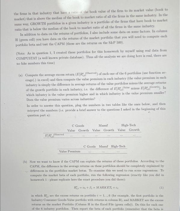
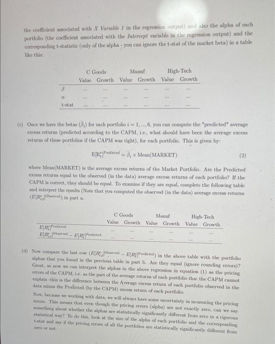
In class we discussed some empirical evidence regarding how the CAPM performs in practice. In addition, we also discussed that in the real world there is a "Value Premium" (as explained in the previous question). In this question I want you to investigate two things: (a) does the value premium varies across industries (ic. is it bigger/smaller in some industries relative to others), and (b) does the CAPM explain the difference in the average returns (i.c. capture the value premium within industries) of these portfolios? In order to answer these questions please open again the Excel data file: Industry Value_Data V2.xlsx, and take a look at the second worksheet with title Industry Portfolios". In this worksheet, you have data with the eccess monthly returns (ie. RR-, and in percentage, so, different from question 1, these are now crcess returns, in excess of the risk free rate) for 6 portfolios for 3 industries. The 3 industries are: (1) Consumer Goods, (2) Manufacturing, and (3) High Tech. For each Industry, I created 2 portfolios: Value and Growth. The firms in the VALUE portfolios in a given industry is a portfolio of the firms in that industry that have a ratio of the book value of the firm to its market value (book to market) that is above the median of the book to market ratio of all the firms in the same industry. In the same way, GROWTH portfolios in a given industry is a portfolio of the firms that have book to market ratio that is below the median of the book to market ratio of all the firms in the same industry, In addition to data on the returns of portfolios, I also include some data on some factors. In column H (green cell) you have data on the returns of the market portfolio that you will need to compute cach portfolio beta and test the CAPM (these are the returns on the S&P 500). (Note: As in question 1. 1 created these portfolios for this homework by myself using real data from COMPUSTAT (a well known private database). Thus all the analysis we are doing here is real, there are no fake mmbers this time) (n) Compute the average excess return (E[R]Observed) of each one of the 6 portfolios (use function - crage() in excel) and then compute the value premium in each industry (the value premium in each industry is simply the difference in average returns of the value portfolios minus the average returns of the growth portfolio in each industry, i.e. the difference of E[R] Value minus EREGrowth). In which industry is the value premium higher and in which industry is the value premium smaller? Does the value premium varies across industries? In order to answer this question, plug the numbers in two tables like the ones below, and then interpret the numbers (ie provide a brief answer to the questions I asked in the beginning of this question parta); C Goods Manur High-Tech ValueGrowth Value Growth Value Growth ERO 06rved * C Goods Manuf High-Tech Value Premium (b) Now we want to know if the CAPM can explain the returns of these portfolios According to the CAPM, the difference in the average returns on these portfolios should be completely explained by differences in the portfolios market betas. To examine this we need to run some regressions. To compute the market beta of each portfolio, run the following regression (exactly file you did in homework 1 - please replicate here the exact procedure you did there): R1=+3MARKET, +41 (1) in which are the excess returns on portfolio 1 = 1.6 (for example, the first portfolio is the Industry Consumer Goods-Value portfolio with returns in column B), and MARKET ate the exces returns on the market Portfolio (Column H in the Excel File (green cells). Do this for each one of the industry portfolion. Then report the both of each portfolio (remember that the beta is X the coefficient Associated with X Variable I in the regression output) and also the alpha of ench portfolio (the coefficient associated with the intercept variable in the regression output) and the corresponding t-statistic (only of the alpha- you can ignore the t-stat of the market beta) in a table like this: C Goods Mam High-Tech Value Growth ValueGrowth Value Growth 8 t-stat (c) Once we have the betas (B) for each portfolio i = 1,...,6, you can compute the predicted" average excess returns (predicted according to the CAPM. i.e., what should have been the average excess returns of these portfolios if the CAPM was right), for each portfolio. This is given by: ER del = 8 x Mean(MARKET) (2) where Mean(MARKET) is the average excess returns of the Market Portfolio. Are the Predicted excess returns equal to the observed in the data) average excess returns of each portfolio? If the CAPM is correct, they should be equal. To examine if they are equal, complete the following table and interpret the results Note that you computed the observed (in the data) average excess returns (E[ Revel) in parta C Goods Manuf High-Tech ValueGrowth Value Growth Value Growth E[ Red ERE, well-E Rebited (d) Now compare the last row (E[ Revel - E|R|Predicted) in the above table with the portfolio alplans that you found in the previous table in part b. Are they equal Ginore rounding errors)? Great, so now we can interpret the alphas in the above regression in equation (1) as the pricing errors of the CAPM. i.e. as the part of the average returns of each portfolio that the CAPM cannot explain this is the difference between the Average excess return of each portfolio observed in the data mims the Predicted by the CAPM) excess return of each portfolio Now, because we worling with data, we will always have some uncertainty in measuring the pricing errors. This means that even though the pricing crons (alpha) are not exactly zero, can we say something about whether the alphas are statistically significantly different from zero in a rigorous statistical way? To do this look at the size of the alpha of each portfolio and the corresponding stat and say if the pricing errors of all the portfolios are statistically significantly different from er or not In class we discussed some empirical evidence regarding how the CAPM performs in practice. In addition, we also discussed that in the real world there is a "Value Premium" (as explained in the previous question). In this question I want you to investigate two things: (a) does the value premium varies across industries (ic. is it bigger/smaller in some industries relative to others), and (b) does the CAPM explain the difference in the average returns (i.c. capture the value premium within industries) of these portfolios? In order to answer these questions please open again the Excel data file: Industry Value_Data V2.xlsx, and take a look at the second worksheet with title Industry Portfolios". In this worksheet, you have data with the eccess monthly returns (ie. RR-, and in percentage, so, different from question 1, these are now crcess returns, in excess of the risk free rate) for 6 portfolios for 3 industries. The 3 industries are: (1) Consumer Goods, (2) Manufacturing, and (3) High Tech. For each Industry, I created 2 portfolios: Value and Growth. The firms in the VALUE portfolios in a given industry is a portfolio of the firms in that industry that have a ratio of the book value of the firm to its market value (book to market) that is above the median of the book to market ratio of all the firms in the same industry. In the same way, GROWTH portfolios in a given industry is a portfolio of the firms that have book to market ratio that is below the median of the book to market ratio of all the firms in the same industry, In addition to data on the returns of portfolios, I also include some data on some factors. In column H (green cell) you have data on the returns of the market portfolio that you will need to compute cach portfolio beta and test the CAPM (these are the returns on the S&P 500). (Note: As in question 1. 1 created these portfolios for this homework by myself using real data from COMPUSTAT (a well known private database). Thus all the analysis we are doing here is real, there are no fake mmbers this time) (n) Compute the average excess return (E[R]Observed) of each one of the 6 portfolios (use function - crage() in excel) and then compute the value premium in each industry (the value premium in each industry is simply the difference in average returns of the value portfolios minus the average returns of the growth portfolio in each industry, i.e. the difference of E[R] Value minus EREGrowth). In which industry is the value premium higher and in which industry is the value premium smaller? Does the value premium varies across industries? In order to answer this question, plug the numbers in two tables like the ones below, and then interpret the numbers (ie provide a brief answer to the questions I asked in the beginning of this question parta); C Goods Manur High-Tech ValueGrowth Value Growth Value Growth ERO 06rved * C Goods Manuf High-Tech Value Premium (b) Now we want to know if the CAPM can explain the returns of these portfolios According to the CAPM, the difference in the average returns on these portfolios should be completely explained by differences in the portfolios market betas. To examine this we need to run some regressions. To compute the market beta of each portfolio, run the following regression (exactly file you did in homework 1 - please replicate here the exact procedure you did there): R1=+3MARKET, +41 (1) in which are the excess returns on portfolio 1 = 1.6 (for example, the first portfolio is the Industry Consumer Goods-Value portfolio with returns in column B), and MARKET ate the exces returns on the market Portfolio (Column H in the Excel File (green cells). Do this for each one of the industry portfolion. Then report the both of each portfolio (remember that the beta is X the coefficient Associated with X Variable I in the regression output) and also the alpha of ench portfolio (the coefficient associated with the intercept variable in the regression output) and the corresponding t-statistic (only of the alpha- you can ignore the t-stat of the market beta) in a table like this: C Goods Mam High-Tech Value Growth ValueGrowth Value Growth 8 t-stat (c) Once we have the betas (B) for each portfolio i = 1,...,6, you can compute the predicted" average excess returns (predicted according to the CAPM. i.e., what should have been the average excess returns of these portfolios if the CAPM was right), for each portfolio. This is given by: ER del = 8 x Mean(MARKET) (2) where Mean(MARKET) is the average excess returns of the Market Portfolio. Are the Predicted excess returns equal to the observed in the data) average excess returns of each portfolio? If the CAPM is correct, they should be equal. To examine if they are equal, complete the following table and interpret the results Note that you computed the observed (in the data) average excess returns (E[ Revel) in parta C Goods Manuf High-Tech ValueGrowth Value Growth Value Growth E[ Red ERE, well-E Rebited (d) Now compare the last row (E[ Revel - E|R|Predicted) in the above table with the portfolio alplans that you found in the previous table in part b. Are they equal Ginore rounding errors)? Great, so now we can interpret the alphas in the above regression in equation (1) as the pricing errors of the CAPM. i.e. as the part of the average returns of each portfolio that the CAPM cannot explain this is the difference between the Average excess return of each portfolio observed in the data mims the Predicted by the CAPM) excess return of each portfolio Now, because we worling with data, we will always have some uncertainty in measuring the pricing errors. This means that even though the pricing crons (alpha) are not exactly zero, can we say something about whether the alphas are statistically significantly different from zero in a rigorous statistical way? To do this look at the size of the alpha of each portfolio and the corresponding stat and say if the pricing errors of all the portfolios are statistically significantly different from er or not