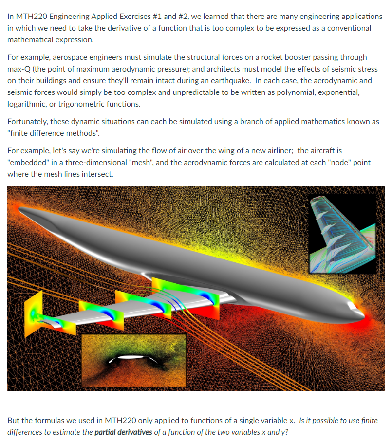
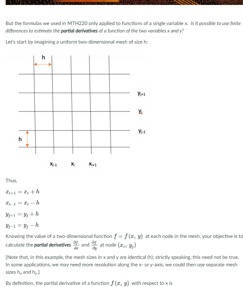
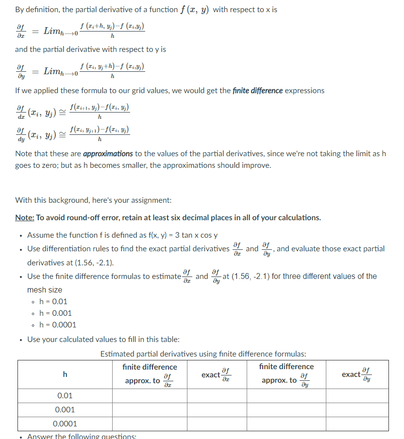
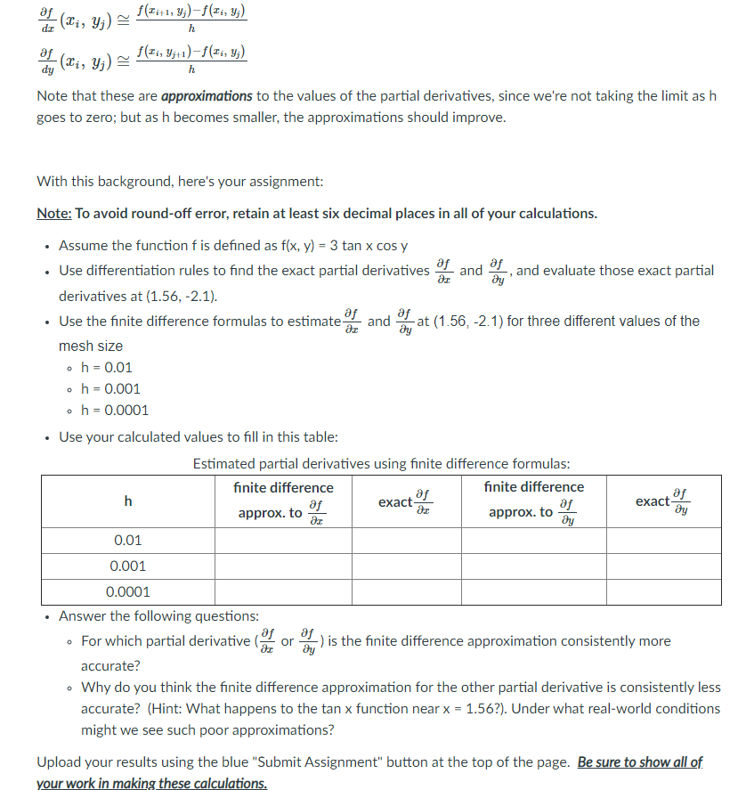
In MTHZEU Engineering Applied Exercises #1 and #2, we learned that there are many engineering applications in which we need to take the derivative of a function that is too complex to be expressed as a conventional mathematical expression. For example, aerospace engineers must simulate the structural forces on a rocket booster passing through maxQ {the point of maximum aerodynamic pressure}; and architects must model the effects of seismic stress on their buildings and ensure thev'll remain intact during an earthquake. In each case, the aerodynamic and seismic forces would simplv be too complex and unpredictable to be written as polynomial, exponential, logarithmic, or trigonometric functions. Fortunately, these dvnamic situations can each be simulated using a branch of applied mathematics known as "finite difference methods". For example, let's say we're simulating the flow of air over the wing of a new airliner; the aircraft is "embedded" in a threedimensional "mesh", and the aerodvnamic forces are calculated at each "node" point where the mesh lines intersect. But the formulas we used in MTHZEG onlyr applied to functions of a single variable x. is it possible to use nite differences to estimate the partial derivatives of a function of the two variables x and v? But the formulas we used in MTH220 only applied to functions of a single variable x. Is it possible to use finite differences to estimate the partial derivatives of a function of the two variables x and y? Let's start by imagining a uniform two-dimensional mesh of size h: Vi+1 yi Vj-1 Xi-1 Xi Xi+1 Thus, Citl = lith Ci-1 = ci - h yit1 = yj th yj-1 = yj - h Knowing the value of a two-dimensional function f = f (x, y) at each node in the mesh, your objective is to calculate the partial derivatives " and " at node (x;, yj) [Note that, in this example, the mesh sizes in x and y are identical (h); strictly speaking, this need not be true. In some applications, we may need more resolution along the x- or y-axis; we could then use separate mesh sizes hx and hy.] By definition, the partial derivative of a function f (x, y) with respect to x isBy definition, the partial derivative of a function f (x, y) with respect to x is - = Limn-+0- f ( Jith, y;) -f (1i,3;) h and the partial derivative with respect to y is dy - = Limn-+0- f ( Ii, y; th)-f (15,y;) If we applied these formula to our grid values, we would get the finite difference expressions h h Note that these are approximations to the values of the partial derivatives, since we're not taking the limit as h goes to zero; but as h becomes smaller, the approximations should improve. With this background, here's your assignment: Note: To avoid round-off error, retain at least six decimal places in all of your calculations. . Assume the function f is defined as f(x, y) = 3 tan x cos y . Use differentiation rules to find the exact partial derivatives of of and , and evaluate those exact partial derivatives at (1.56, -2.1). . Use the finite difference formulas to estimate of " and " at (1.56, -2.1) for three different values of the mesh size o h = 0.01 o h = 0.001 o h = 0.0001 . Use your calculated values to fill in this table: Estimated partial derivatives using finite difference formulas: finite difference h of finite difference exact exact- approx. to approx. to- of 0.01 0.001 0.0001of (ci, yj) h (Xi, yi) ~ (zijl) -f(Ii, y;) h Note that these are approximations to the values of the partial derivatives, since we're not taking the limit as h goes to zero; but as h becomes smaller, the approximations should improve. With this background, here's your assignment: Note: To avoid round-off error, retain at least six decimal places in all of your calculations. . Assume the function f is defined as f(x, y) = 3 tan x cos y . Use differentiation rules to find the exact partial derivatives _ and , and evaluate those exact partial derivatives at (1.56, -2.1). . Use the finite difference formulas to estimate of Of and By of at (1.56, -2.1) for three different values of the mesh size o h = 0.01 o h = 0.001 o h = 0.0001 Use your calculated values to fill in this table: Estimated partial derivatives using finite difference formulas: finite difference finite difference h approx. to- of exact of of approx. to y exact Dy 0.01 0.001 0.0001 Answer the following questions: . For which partial derivative (as or @ ) is the finite difference approximation consistently more accurate? . Why do you think the finite difference approximation for the other partial derivative is consistently less accurate? (Hint: What happens to the tan x function near x = 1.56?). Under what real-world conditions might we see such poor approximations? Upload your results using the blue "Submit Assignment" button at the top of the page. Be sure to show all of. your work in making these calculations