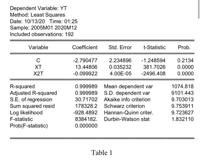
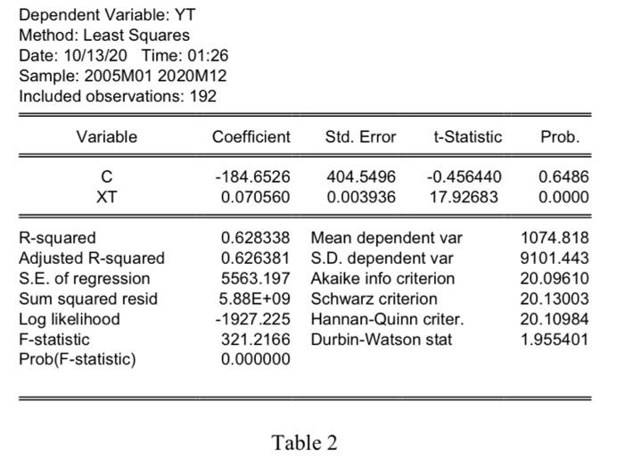
In Table 1, we report the estimated model where Yt is the wage of CEOs, Xt is the age of them and X2t is the squared value of Xt. The model is estimated using EViews, 1) Watch Video about Quadratic Terms in Extra Videos. 2) Do you think the regression is a good regression? (Look at the R2, F statistic, and t statistics). 3) Calculate the impact of the age on the wage of CEOs. Discuss the quadratic effect. 4) In Table 2, we re-estimate the model without the quadratic term but considering the dependent variable transformed using natural logarithm. After watching the Video LogVsLevel in Extra Videos, comment on the results. Define the marginal effect and the elasticity in the average point considering (in addition to information you have in Table 2) that the mean of X is 55. Dependent Variable: YT Method: Least Squares Date: 10/13/20 Time: 01:25 Sample: 2005M01 2020M12 Included observations: 192 Variable Coefficient Std. Error t-Statistic Prob. XT X2T -2.790477 13.44806 -0.099922 2.234896 0.035232 4.00E-05 -1.248594 381.7026 -2496.408 0.2134 0.0000 0.0000 R-squared Adjusted R-squared S.E. of regression Sum squared resid Log likelihood F-statistic Prob(F-statistic) 0.999989 Mean dependent var 0.999989 S.D. dependent var 30.71702 Akaike info criterion 178328.2 Schwarz criterion -928.4892 Hannan-Quinn criter. 8384 182. Durbin-Watson stat 0.000000 1074.818 9101.443 9.703013 9.753911 9.723627 1.832110 Table 1 Dependent Variable: YT Method: Least Squares Date: 10/13/20 Time: 01:26 Sample: 2005M01 2020M12 Included observations: 192 Variable Coefficient Std. Error t-Statistic Prob. XT -184.6526 0.070560 404.5496 0.003936 -0.456440 17.92683 0.6486 0.0000 R-squared Adjusted R-squared S.E. of regression Sum squared resid Log likelihood F-statistic Prob(F-statistic) 0.628338 Mean dependent var 0.626381 S.D. dependent var 5563.197 Akaike info criterion 5.88E+09 Schwarz criterion -1927.225 Hannan-Quinn criter. 321.2166 Durbin-Watson stat 0.000000 1074.818 9101.443 20.09610 20.13003 20.10984 1.955401 Table 2 In Table 1, we report the estimated model where Yt is the wage of CEOs, Xt is the age of them and X2t is the squared value of Xt. The model is estimated using EViews, 1) Watch Video about Quadratic Terms in Extra Videos. 2) Do you think the regression is a good regression? (Look at the R2, F statistic, and t statistics). 3) Calculate the impact of the age on the wage of CEOs. Discuss the quadratic effect. 4) In Table 2, we re-estimate the model without the quadratic term but considering the dependent variable transformed using natural logarithm. After watching the Video LogVsLevel in Extra Videos, comment on the results. Define the marginal effect and the elasticity in the average point considering (in addition to information you have in Table 2) that the mean of X is 55. Dependent Variable: YT Method: Least Squares Date: 10/13/20 Time: 01:25 Sample: 2005M01 2020M12 Included observations: 192 Variable Coefficient Std. Error t-Statistic Prob. XT X2T -2.790477 13.44806 -0.099922 2.234896 0.035232 4.00E-05 -1.248594 381.7026 -2496.408 0.2134 0.0000 0.0000 R-squared Adjusted R-squared S.E. of regression Sum squared resid Log likelihood F-statistic Prob(F-statistic) 0.999989 Mean dependent var 0.999989 S.D. dependent var 30.71702 Akaike info criterion 178328.2 Schwarz criterion -928.4892 Hannan-Quinn criter. 8384 182. Durbin-Watson stat 0.000000 1074.818 9101.443 9.703013 9.753911 9.723627 1.832110 Table 1 Dependent Variable: YT Method: Least Squares Date: 10/13/20 Time: 01:26 Sample: 2005M01 2020M12 Included observations: 192 Variable Coefficient Std. Error t-Statistic Prob. XT -184.6526 0.070560 404.5496 0.003936 -0.456440 17.92683 0.6486 0.0000 R-squared Adjusted R-squared S.E. of regression Sum squared resid Log likelihood F-statistic Prob(F-statistic) 0.628338 Mean dependent var 0.626381 S.D. dependent var 5563.197 Akaike info criterion 5.88E+09 Schwarz criterion -1927.225 Hannan-Quinn criter. 321.2166 Durbin-Watson stat 0.000000 1074.818 9101.443 20.09610 20.13003 20.10984 1.955401 Table 2


