In the excel please thank you

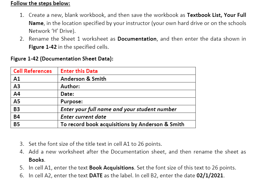
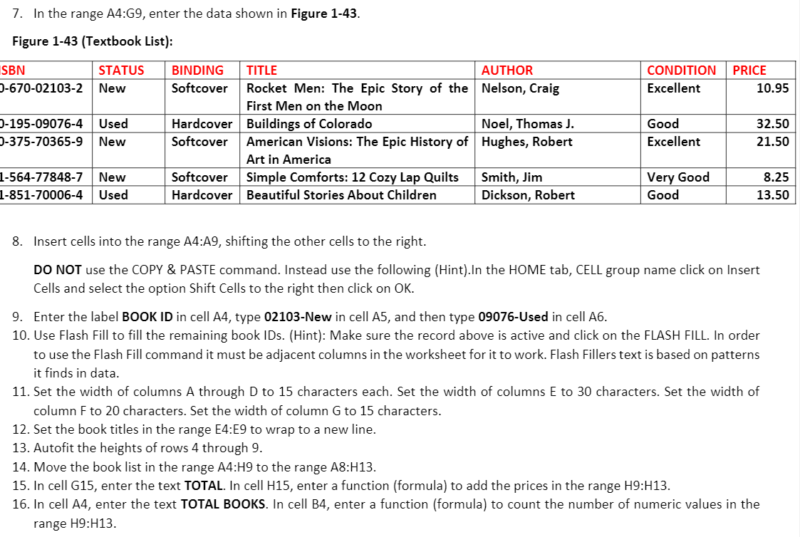
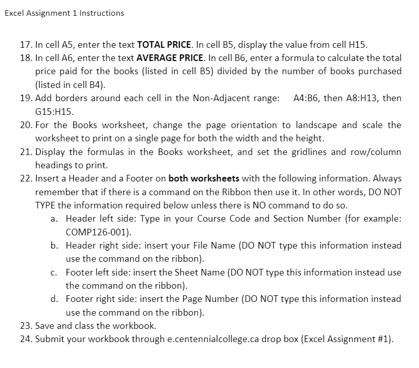
Follow the steps below: 1. Create a new, blank workbook, and then save the workbook as Textbook List, Your Full Name, in the location specified by your instructor (your own hard drive or on the schools Network 'H' Drive). 2. Rename the Sheet 1 worksheet as Documentation, and then enter the data shown in Figure 1-42 in the specified cells. Figure 1-42 (Documentation Sheet Data): Cell References A1 A3 A4 A5 B3 B4 B5 Enter this Data Anderson & Smith Author: Date: Purpose: Enter your full name and your student number Enter current date To record book acquisitions by Anderson & Smith 3. Set the font size of the title text in cell A1 to 26 points. 4. Add a new worksheet after the Documentation sheet, and then rename the sheet as Books. 5. In cell A1, enter the text Book Acquisitions. Set the font size of this text to 26 points. 6. In cell A2, enter the text DATE as the label. In cell B2, enter the date 02/1/2021. 7. In the range A4:39, enter the data shown in Figure 1-43. Figure 1-43 (Textbook List): ISBN 0-670-02103-2 STATUS New CONDITION Excellent PRICE 10.95 0-195-09076-4 0-375-70365-9 Used New BINDING TITLE AUTHOR Softcover Rocket Men: The Epic Story of the Nelson, Craig First Men on the Moon Hardcover Buildings of Colorado Noel, Thomas J. Softcover American Visions: The Epic History of Hughes, Robert Art in America Softcover Simple Comforts: 12 Cozy Lap Quilts Smith, Jim Hardcover Beautiful Stories About Children Dickson, Robert Good Excellent 32.50 21.50 1-564-77848-7 1-851-70006-4 New Used Very Good Good 8.25 13.50 8. Insert cells into the range A4:19, shifting the other cells to the right. DO NOT use the COPY & PASTE command. Instead use the following (Hint). In the HOME tab, CELL group name click on Insert Cells and select the option Shift Cells to the right then click on OK. 9. Enter the label BOOK ID in cell A4, type 02103-New in cell AS, and then type 09076-Used in cell A6. 10. Use Flash Fill to fill the remaining book IDs. (Hint): Make sure the record above is active and click on the FLASH FILL. In order to use the Flash Fill command it must be adjacent columns in the worksheet for it to work. Flash Fillers text is based on patterns it finds in data. 11. Set the width of columns A through D to 15 characters each. Set the width of columns E to 30 characters. Set the width of column F to 20 characters. Set the width of column G to 15 characters. 12. Set the book titles in the range E4:E9 to wrap to a new line. 13. Autofit the heights of rows 4 through 9. 14. Move the book list in the range A4:H9 to the range A8:H13. 15. In cell G15, enter the text TOTAL. In cell H15, enter a function (formula) to add the prices in the range H9:H13. 16. In cell A4, enter the text TOTAL BOOKS. In cell B4, enter a function (formula) to count the number of numeric values in the range H9:H13. Excel Assignment 1 Instructions 17. In cell A5, enter the text TOTAL PRICE. In cell B5, display the value from cell H15. 18. In cell A6, enter the text AVERAGE PRICE. In cell B6, enter a formula to calculate the total price paid for the books (listed in cell B5) divided by the number of books purchased (listed in cell B4). 19. Add borders around each cell in the Non-Adjacent range: A4:B6, then A8:H13, then G15:H15. 20. For the Books worksheet, change the page orientation to landscape and scale the worksheet to print on a single page for both the width and the height. 21. Display the formulas in the Books worksheet, and set the gridlines and row/column headings to print. 22. Insert a Header and a Footer on both worksheets with the following information. Always remember that if there is a command on the Ribbon then use it. In other words, DO NOT TYPE the information required below unless there is NO command to do so. a. Header left side: Type in your Course Code and Section Number (for example: COMP126-001). b. Header right side: insert your File Name (DO NOT type this information instead use the command on the ribbon). C. Footer left side: insert the Sheet Name (DO NOT type this information instead use the command on the ribbon). d. Footer right side: insert the Page Number (DO NOT type this information instead use the command on the ribbon). 23. Save and class the workbook. 24. Submit your workbook through e.centennialcollege.ca drop box (Excel Assignment #1). Follow the steps below: 1. Create a new, blank workbook, and then save the workbook as Textbook List, Your Full Name, in the location specified by your instructor (your own hard drive or on the schools Network 'H' Drive). 2. Rename the Sheet 1 worksheet as Documentation, and then enter the data shown in Figure 1-42 in the specified cells. Figure 1-42 (Documentation Sheet Data): Cell References A1 A3 A4 A5 B3 B4 B5 Enter this Data Anderson & Smith Author: Date: Purpose: Enter your full name and your student number Enter current date To record book acquisitions by Anderson & Smith 3. Set the font size of the title text in cell A1 to 26 points. 4. Add a new worksheet after the Documentation sheet, and then rename the sheet as Books. 5. In cell A1, enter the text Book Acquisitions. Set the font size of this text to 26 points. 6. In cell A2, enter the text DATE as the label. In cell B2, enter the date 02/1/2021. 7. In the range A4:39, enter the data shown in Figure 1-43. Figure 1-43 (Textbook List): ISBN 0-670-02103-2 STATUS New CONDITION Excellent PRICE 10.95 0-195-09076-4 0-375-70365-9 Used New BINDING TITLE AUTHOR Softcover Rocket Men: The Epic Story of the Nelson, Craig First Men on the Moon Hardcover Buildings of Colorado Noel, Thomas J. Softcover American Visions: The Epic History of Hughes, Robert Art in America Softcover Simple Comforts: 12 Cozy Lap Quilts Smith, Jim Hardcover Beautiful Stories About Children Dickson, Robert Good Excellent 32.50 21.50 1-564-77848-7 1-851-70006-4 New Used Very Good Good 8.25 13.50 8. Insert cells into the range A4:19, shifting the other cells to the right. DO NOT use the COPY & PASTE command. Instead use the following (Hint). In the HOME tab, CELL group name click on Insert Cells and select the option Shift Cells to the right then click on OK. 9. Enter the label BOOK ID in cell A4, type 02103-New in cell AS, and then type 09076-Used in cell A6. 10. Use Flash Fill to fill the remaining book IDs. (Hint): Make sure the record above is active and click on the FLASH FILL. In order to use the Flash Fill command it must be adjacent columns in the worksheet for it to work. Flash Fillers text is based on patterns it finds in data. 11. Set the width of columns A through D to 15 characters each. Set the width of columns E to 30 characters. Set the width of column F to 20 characters. Set the width of column G to 15 characters. 12. Set the book titles in the range E4:E9 to wrap to a new line. 13. Autofit the heights of rows 4 through 9. 14. Move the book list in the range A4:H9 to the range A8:H13. 15. In cell G15, enter the text TOTAL. In cell H15, enter a function (formula) to add the prices in the range H9:H13. 16. In cell A4, enter the text TOTAL BOOKS. In cell B4, enter a function (formula) to count the number of numeric values in the range H9:H13. Excel Assignment 1 Instructions 17. In cell A5, enter the text TOTAL PRICE. In cell B5, display the value from cell H15. 18. In cell A6, enter the text AVERAGE PRICE. In cell B6, enter a formula to calculate the total price paid for the books (listed in cell B5) divided by the number of books purchased (listed in cell B4). 19. Add borders around each cell in the Non-Adjacent range: A4:B6, then A8:H13, then G15:H15. 20. For the Books worksheet, change the page orientation to landscape and scale the worksheet to print on a single page for both the width and the height. 21. Display the formulas in the Books worksheet, and set the gridlines and row/column headings to print. 22. Insert a Header and a Footer on both worksheets with the following information. Always remember that if there is a command on the Ribbon then use it. In other words, DO NOT TYPE the information required below unless there is NO command to do so. a. Header left side: Type in your Course Code and Section Number (for example: COMP126-001). b. Header right side: insert your File Name (DO NOT type this information instead use the command on the ribbon). C. Footer left side: insert the Sheet Name (DO NOT type this information instead use the command on the ribbon). d. Footer right side: insert the Page Number (DO NOT type this information instead use the command on the ribbon). 23. Save and class the workbook. 24. Submit your workbook through e.centennialcollege.ca drop box (Excel Assignment #1)