In this chapter we are looking at the differential equations that govern RC circuits. For a capacitor that is discharging, we know that going around the circuit the voltage should sum to zero:

Vc + Vr = 0.

Written in terms of charge and current, this is:

q/C = - i R.

Rewritten,

q/C = -dq/dt R.

What this is telling us is that the current is being set by the charge on the capacitor. We can use a numerical approach to model this system. We know that dq/dt is a change in charge divided by a change in time:

q/t or (qf-qi)/t,

where qi is the initial charge and qf is the final charge.

Treating q as qi, this allows us to state:

qi/C = -[(qf-qi)/t] (1/R).

Solving for qf, we get:

qf = qi (qi/RC) t.

qf = qi (1 t/RC).

In other words, at each small step in time, we subtract off a value proportional to the current charge.

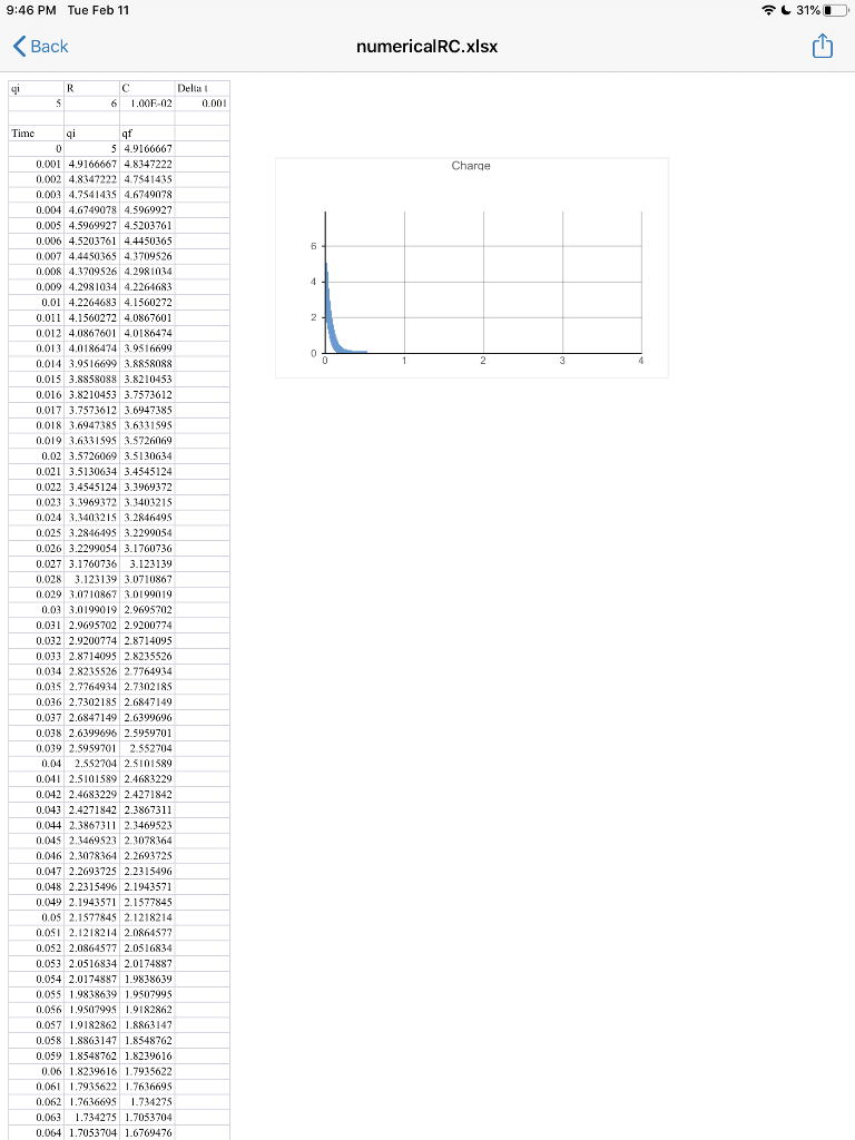
We can model this behavior in a spreadsheet. Well use some tricks to help us out. In the top of the spreadsheet well define four quantities: t, R, C and qi. This gives us details of the circuit and also the change in time. I put in some sample values, feel free to change them in order to experiment with how circuits work.

We then set up three columns. The first is a time column, the second is qi and the third is qf. Lets look at first row. Time initial is zero, charge initial is set by the variables at the top of the chart and qf is done by formula, it is qi multiplied by (1t/RC). Note that these values use absolute relationships, eg. $B$2, so if the formula gets copied, then it always refers back to the values at the top of the chart.

The next line down is really the key to the whole affair. The time column is the time from the line above, plus the delta t. The qi is the qf from the previous line, and the qf is calculated from the qi on this line. Note that since so many of the entries are in reference to the previous line, we can simply copy this expression to the line below to now have a three-step process. In fact, we can do this repeatedly (I did it 500 times) to watch how q changes from step-to-step in time. I graphed the q(t) behavior, and you can see it is an exponential, just as predicted by theory.

For this weeks homework, add a battery to this circuit and make a new spreadsheet that corresponds to charging up an empty capacitor. Your spreadsheet should include the appropriate graph. Note that for things like RC circuits, it is usually simpler to just solve the differential equation. For more complex problems, scientists and engineers will often use numerical methods rather than directly tackle hard math problems.

Note that you will need to submit an Excel file, not a picture. The file should have step-by-step charging, modeled on the sample spreadsheet. Simply having Excel graph an exponential will not satisfy this assignment.

Download the following Excel file and then modify it so that it does a numerical simulation of a charging capacitor. Then upload your new file. This is what the excel file looks like:

9:46 PM Tue Feb 11 31%D