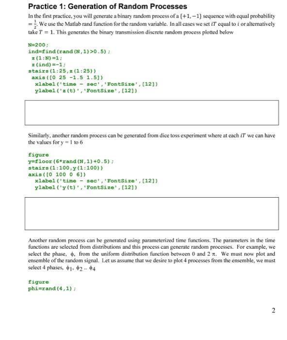
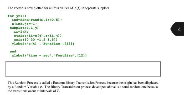
In this exercise, you will compute the correlation function for Random Processes that contain sinusoidal functions of time. X(t) = Acos( t) - Bsin(wit) where A and B are two random variables. Find the R(t, 1+T)= E[X(t)X(t,t+r)] and then find the conditions upon E[A], E[B], E[A], E[B] and the E[AB] to make the process X(t) is a wide sense stationary. Practice 1: Generation of Random Processes In the first practice, you will generate a binary random process of a (+1,-1] sequence with equal probability = We use the Matlab rand function for the random variable. In all cases we set iT equal to i or alternatively take T = 1. This generates the binary transmission discrete random process plotted below N=200; ind=find (rand (N, 1) >0.5); z (1:N)=1; z (ind) = -1; stairs (1:25, z (1:25)) axis ( [0 25 -1.5 1.51) xlabel (time ylabel ('z(t)', 'FontSize', [12]). sec', 'FontSize', [12]) Similarly, another random process can be generated from dice toss experiment where at each iT we can have the values for y = 1 to 6 figure y=floor (6*rand (N, 1) +0.5); stairs (1:100,y (1:100)) axis ( [0 100 0 6]) xlabel ('time - sec', 'FontSize', [12]) ylabel ('y(t)', 'FontSize', [12]) Another random process can be generated using parameterized time functions. The parameters in the time functions are selected from distributions and this process can generate random processes. For example, we select the phase, , from the uniform distribution function between 0 and 2n. We must now plot and ensemble of the random signal. Let us assume that we desire to plot 4 processes from the ensemble, we must select 4 phases, 1.92-94 figure phi=rand (4,1); The four Random Processes can now be generated using the selected phases as x(i.) = cos(0.1 +2-pi-phi()) The plot below graphs the 4 ensemble functions each in a subgraph for clarity for j=1:4 for i=1:N x (1,3)=cos (.1*1+2*pi*phi (j)); end subplot (4,1, 3) ii=1:100; plot (ii,x(ii,5)) axis ([0 100 -1.5 1.51) ylabel ('y(t)', 'FontSize', [12]) end xlabel('time - sec', 'FontSize', [12]) ylabel ('y(t)', 'FontSize', [12]) The next group of Random Processes is generated by summation of identically and independently distributed (iid) Random Variables at each iT. Summing the Bernoulli (+1.-1) iid Random Variable at each iT forms the waveform as figure a (1)=0; for i=1:100 s(i+1)= (i) + (i); end The s variable is the running sum of the iid Random Variable zj from i = 0 to i. This Random Process is called discrete Random Walk. stairs (s) xlabel('time- sec', 'FontSize', [12]) ylabel ('s(t), 'FontSize', [12]) The Binary Transmission Random Process generated above can be combined with a random parameter to generate another random process. Let us assume that the origin can be displaced by a random Variable, e, that is uniformly distributed in (0.7]. The ensemble function can now be plotted for four values of e,. In order to facilitate the plotting of this process a vector z of all ones is composed. The ind vector contains the components that are changed to -1 by the random vector figure e=rand (4,1); N=50; z=ones (N, 4); W The vector is now plotted for all four values of e(i) in separate subplots for j=1:4 ind=find (rand (N, 1) >0.5); z (ind, j)=-1; subplot (4,1,1) ii=1: N; stairs (ii+e (j),z (ii, j)) axis ( [0 30 -1.5 1.5]) ylabel ('z(t)', 'FontSize', [12]) end xlabel('time sec', 'FontSize', [12]) This Random Process is called a Random Binary Transmission Process because the origin has been displaced by a Random Variable e. The Binary Transmission process developed above is a semi-random one because the transitions occur at intervals of T.