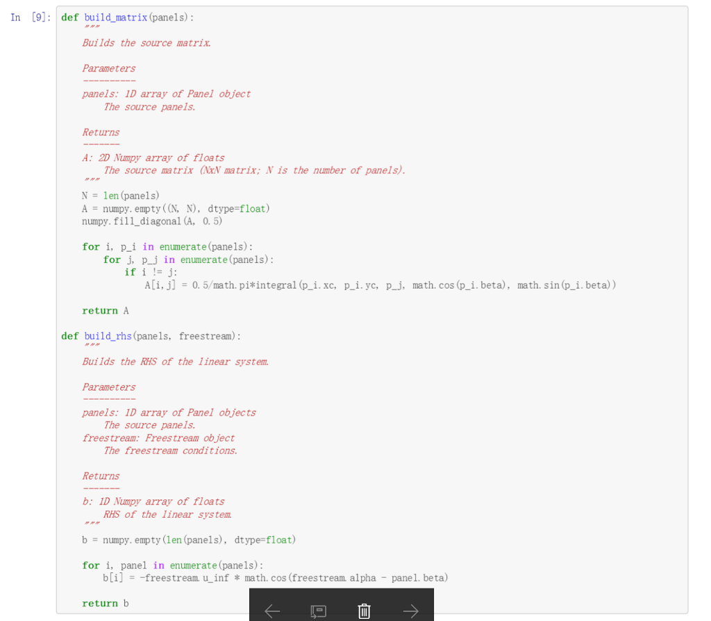
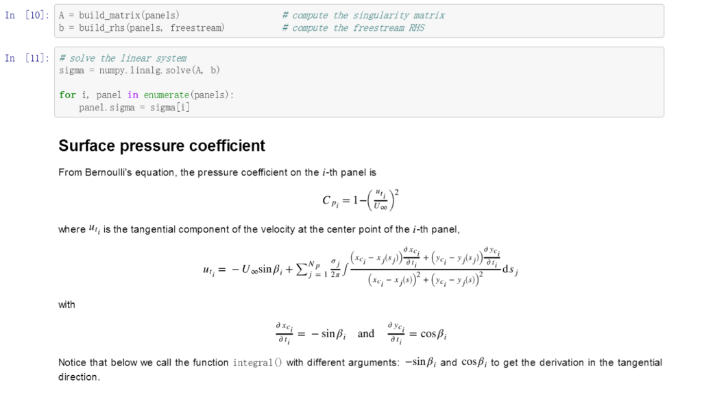
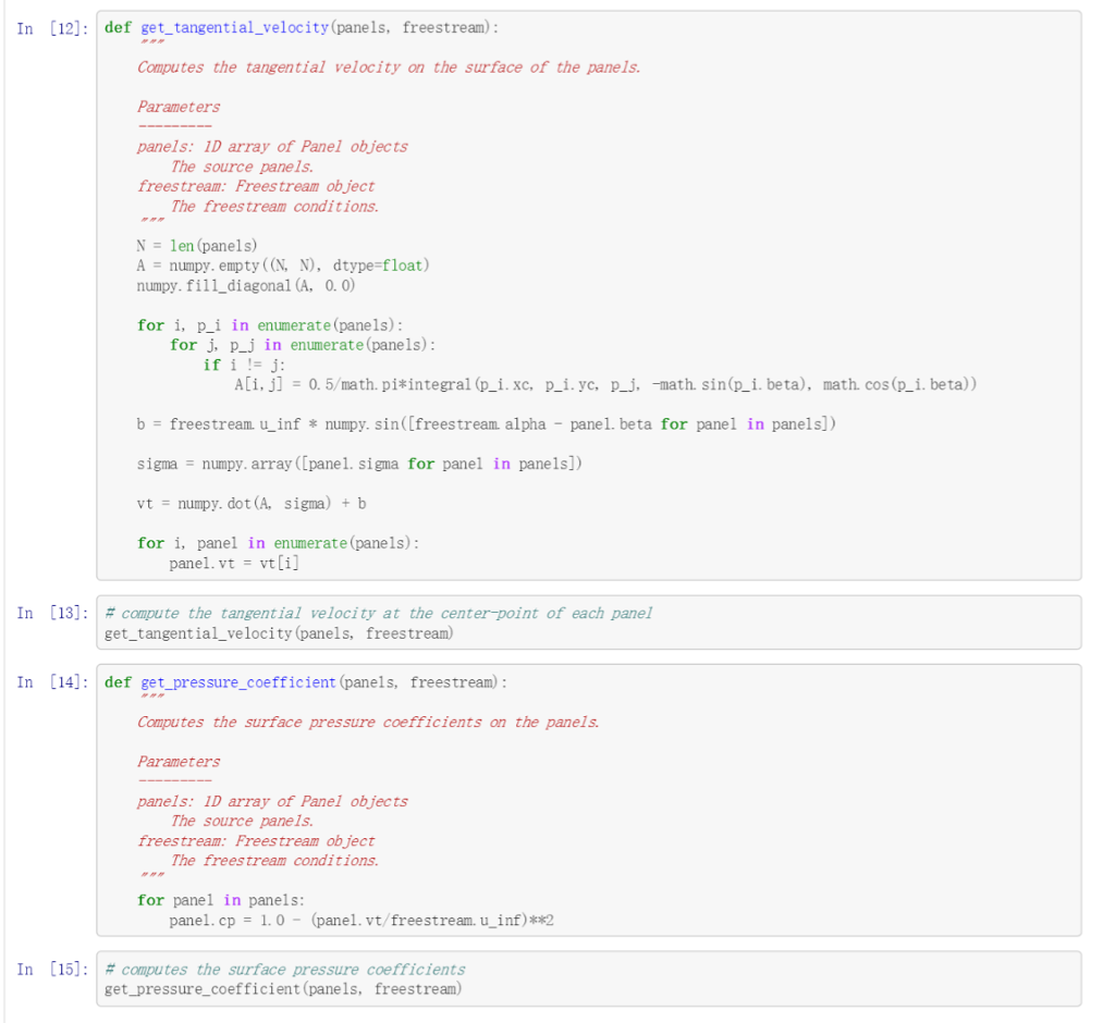
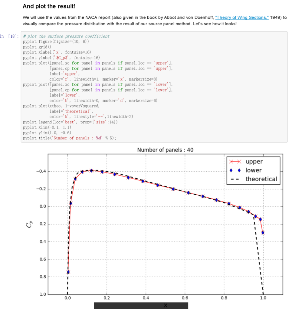
In this picture above, they used constant strength source panel method to analyze the pressure coefficient around the NASA0012 airfoil, please change it to linear strength source panel method based on these codes and release the new code here in python. thank you

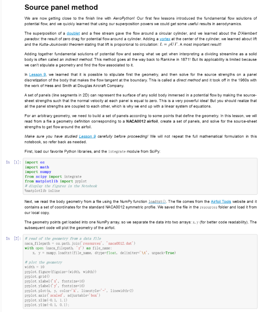
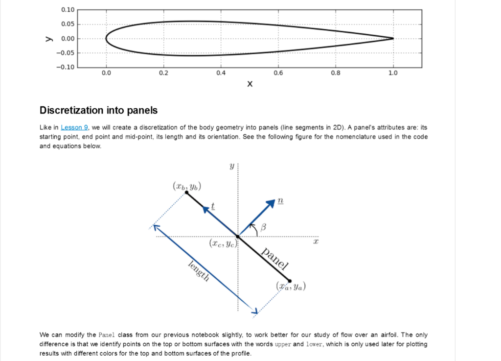
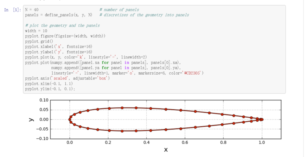
Source panel method We are now getting close to the finish line with AeroPython! Our first few lessons introduced the fundamental flow solutions of potential flow, and we quickly learned that using our superposition powers we could get some useful results in aerodynamics. The superposition of a doublet and a free stream gave the flow around a circular cylinder, and we learned about the D'Alembert paradox the result of zero drag for potential flow around a cylinder. Adding a vortex at the center of the cylinder, we learned about lift and the Kutta-Joukowski theorem stating that lift is proporional to circulation: L J pUT. A most important resul Adding together fundamental solutions of potential flow and seeing what we get when interpreting a dividing streamline as a solid body is often called an indirect method. This method goes all the way back to Rankine in 1871! But its applicability is limited because we can't stipulate a geometry a find the flow associated to it in Lesson 9, we learned that it is possible to stipulate first the geometry, and then solve for the source strengths on a panel discretization of the body that makes the flow tangent at the boundary. This is called a direct method and it took off in the 1960s with the work of Hess and Smith at Douglas Aircraft Company. A set of panels (line segments in 2D) can represent the surface of any solid body immersed in a potential flow by making the source- sheet strengths such that the normal velocity at each panel is equal to zero. This is a very powerful idea! But you should realize that all the panel strengths are coupled to each other, which is why we end up with a linear system of equations. For an arbitrary geometry, we need to build a set of panels according to some points that define the geometry. In this lesson, we will read from a file a geometry definition corresponding to a NACA0012 airfo create a set of panels, and solve for the source-sheet strengths to get flow around the airfoil. Make sure you have studied Lesson 9 carefully before proceeding! We will not repeat the full mathematical formulation in this notebook, so refer back as needed. First, load our favorite Python libraries, and the integrate module from SciPy: In [1]: import oss import math import numpy from scipy import integrate from matplotlib import pyplot display the figures in the Noteboak %matplotlib inline Next, we read the body geometry from a file using the NumPy function loadtxt O. The file comes from the AirfoiITools website and it contains a set of coordinates for the standard NACA0012 symmetric profile. We saved the file in the resources folder and load it from our local copy. The geometry points get loaded into one NumPy array, so we separate the data into two arrays (for better code readability). The X, y subsequent code will plot the geometry of the airfoil. In [2]: read of the geometry from a data file os, path. join resources naca0012, dat') naca filepath. with open (naca filepath, 'r') as file name numpy. loadtxt(file name, dtype float, delimiter lt unpack True) plot the geametry width 10 pyplot. figure (figsize (width, width)) pyplot. grid0 pyplot. label fontsize 16) pyplot. y label y fontsize 16) pyplot. plot (k, y, color linewidth 2) line style pyplot. axis scaled adjustable box pyplot. ylim 0.1, 0.1)