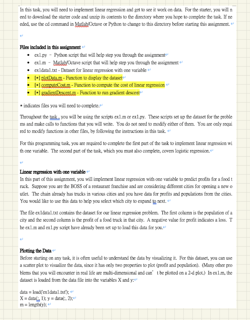
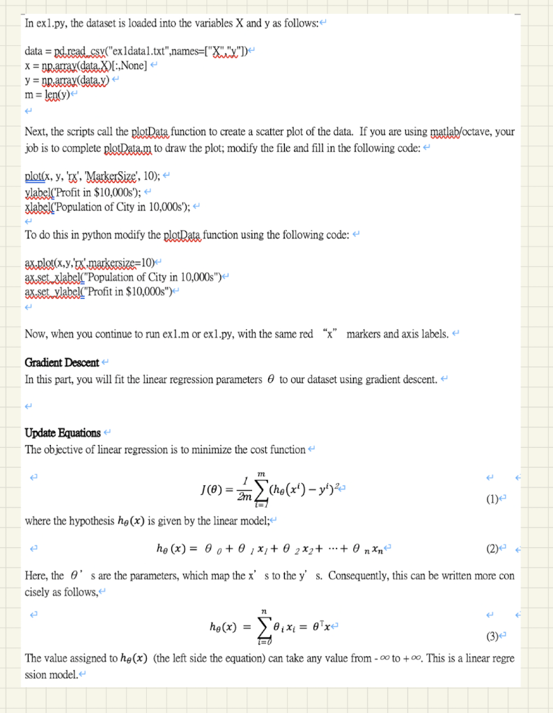
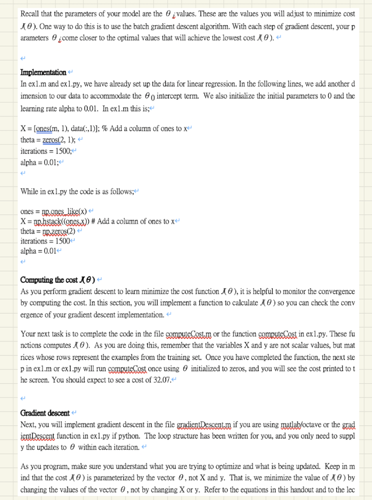
In this task, you will need to implement linear regression and get to see it work on data. For the starter, you will n eed to download the starter code and unzip its contents to the directory where you hope to complete the task. If ne eded, use the cd command in Matlab/Octave or Python to change to this directory before starting this assignment. Files included in this assignment exl.py - Python script that will help step you through the assignment- exl.m - Matlab/Octave script that will help step you through the assignment exldatal.txt - Dataset for linear regression with one variable [*] plotData.m - Function to display the dataset [*] computeCost.m - Function to compute the cost of linear regression [*gradientDescentm - Function to run gradient descent . * indicates files you will need to complete. Throughout the task. you will be using the scripts exl.m or exl.py. These scripts set up the dataset for the proble ms and make calls to functions that you will write. You do not need to modify either of them. You are only requi red to modify functions in other files, by following the instructions in this task. For this programming task, you are required to complete the first part of the task to implement linear regression wi th one variable. The second part of the task, which you must also complete, covers logistic regression. Linear regression with one variable In this part of this assignment, you will implement linear regression with one variable to predict profits for a foodt ruck. Suppose you are the BOSS of a restaurant franchise and are considering different cities for opening a new o utlet. The chain already has trucks in various cities and you have data for profits and populations from the cities. You would like to use this data to help you select which city to expand to next. The file exldatal.txt contains the dataset for our linear regression problem. The first column is the population of a city and the second column is the profit of a food truck in that city. A negative value for profit indicates a loss. T he exl.m and ex1.py script have already been set up to load this data for you. Plotting the Data Before starting on any task, it is often useful to understand the data by visualizing it. For this dataset, you can use a scatter plot to visualize the data, since it has only two properties to plot (profit and population). (Many other pro blems that you will encounter in real life are multi-dimensional and can't be plotted on a 2-d plot.) In ex1.m, the dataset is loaded from the data file into the variables X and y: data = load('exldatal.txt'); X = data: 1); y = data(:, 2); m = length(y); In ex1.py, the dataset is loaded into the variables X and y as follows: data = pd. read csx("exldatal.txt",names=["XX")) X = np.array(data.&)[:,None] y = np.array(data,y) m = len(y) Next, the scripts call the plotData function to create a scatter plot of the data. If you are using matlab/octave, your job is to complete plotData.m to draw the plot; modify the file and fill in the following code: plot(x, y, 'rx', 'MarkerSize', 10); ylabel('Profit in $10,000s'); xlabel('Population of City in 10,000s"); To do this in python modify the plotData function using the following code: ax.plot(x,y,rx',markersize=10)- ax-setuxlabel("Population of City in 10,000s") ax.set_label("Profit in $10,000s") Now, when you continue to run ex1.m or exl.py, with the same red "x" markers and axis labels. Gradient Descent In this part, you will fit the linear regression parameters to our dataset using gradient descent. Update Equations The objective of linear regression is to minimize the cost function m 1 JO)= 2m (h(x)-y) (1) where the hypothesis he(x) is given by the linear model; ho (x) = @o+,x;+ 2x2+ ... + Onxn (2) Here, the e' s are the parameters, which map the x's to the y's. Consequently, this can be written more con cisely as follows, , he(x) = 8 x = 8Txe ied (3) The value assigned to he(x) (the left side the equation) can take any value from - co to +0. This is a linear regre ssion model. Recall that the parameters of your model are the values. These are the values you will adjust to minimize cost 10). One way to do this is to use the batch gradient descent algorithm. With each step of gradient descent, your p arameters come closer to the optimal values that will achieve the lowest cost @). Implementation In exl.m and ex1.py, we have already set up the data for linear regression. In the following lines, we add another d imension to our data to accommodate the intercept term. We also initialize the initial parameters to 0 and the learning rate alpha to 0.01. In exl.m this is;- X = [ones(m, 1), data(:,1)]; % Add a column of ones to x theta = zeros(2, 1); iterations = 1500; alpha = 0.01; While in ex l.py the code is as follows: ones = np.ones like(x) X = ppbstack(ones.x)) # Add a column of ones to x theta = pr.zeros(2) iterations = 1500- alpha = 0.01 Computing the cost 10) As you perform gradient descent to learn minimize the cost function e), it is helpful to monitor the convergence by computing the cost. In this section, you will implement a function to calculate 10) so you can check the conv ergence of your gradient descent implementation. Your next task is to complete the code in the file computeCostum or the function computeCast in exl.py. These fu nctions computes O). As you are doing this, remember that the variables X and y are not scalar values, but mat rices whose rows represent the examples from the training set. Once you have completed the function, the next ste p in exl.m or exl.py will run computeCost once using initialized to zeros, and you will see the cost printed to t he screen. You should expect to see a cost of 32.07.- Gradient descent Next, you will implement gradient descent in the file gradientDescentm if you are using matlab/octave or the grad ientDescent function in exl.py if python. The loop structure has been written for you, and you only need to suppl y the updates to within each iteration. As you program, make sure you understand what you are trying to optimize and what is being updated. Keep in m ind that the cost @) is parameterized by the vector 2, not X and y. That is, we minimize the value of 0) by changing the values of the vector , not by changing X or y. Refer to the equations in this handout and to the lec A good way to verify that gradient descent is working correctly is to look at the value of O) and check that it is decreasing with each step. Assuming you have implemented gradient descent and computeCost correctly, your val ue of 1 ) should never increase, and should converge to a steady value by the end of the algorithm. After you ar e finished, the code will use your final parameters to plot the linear fit. Your final values for will also be used to make predictions on profits in areas of 35,000 and 70,000 people. No te the way that the following lines in exl.m uses matrix multiplication, rather than explicit summation or looping, t o calculate the predictions. This is an example of code vectorization predict1 = [1, 3.5] * theta; predict2 = [1, 7] * theta; These lines in ex1.py are; predictl = np.dot([1, 3.5), theta) predict2 = np.dot([1, 2],theta) Visualizing 10) To understand the cost function () better, you will now plot the cost over a 2-dimensional grid of eo and 1 values. You will not need to code anything new for this part, but you should understand how the code you have wr itten already is creating these images. In the next step of exl.m, there is code set up to calculate 1 e) over a grid of values using the computeCost functi on that you wrote. Lavals = zeros(length(theta_vals), length(thetal_vals)); for i = 1:length(theta_vals) for j = 1:length(thetal_vals) t= [theta_vals(i); thetal_vals()); vals(i.) = computeCost(x, y, t); end end In the python script the code set up to calculate 10) over a grid of values using the computeCost function that yo u wrote is; L vals = np.zeros((len(thetaQ_vals),len(thetal_vals))) for i in range(len(theta_vals): for j in range(len(thetal_vals)): t = np.array( [theta_vals[i],thetal_vals[:]]) Luvals[i][j] = computeCost(X.Xat) After these lines are executed, you will have a 2-D array of 10) values. The code will then use these values to pr oduce surface and contour plots of 10) using the surf and contour commands. 4 The purpose of these graphs is to show you that how (e) varies with changes in 0 and 0 1. The cost function 10) is bowl-shaped and has a global minimum. (This is easier to see in the contour plot than in the 3D surface pl ot). This minimum is the optimal point for @ and @ 1, and each step of gradient descent. Required: a) Using your own words, briefly define the functions computeCost and gradientDescent. b) Create flowchart solutions for computeCost and gradient Descent. c) As BOSS, your goal is to gain strategic advantage over its rival firms. How can the food truck business us e data analytics analytics and exploit social media to accomplish this goal