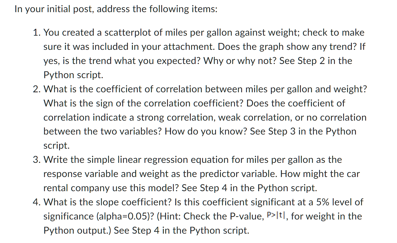
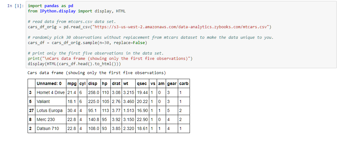
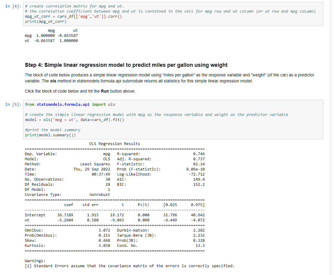
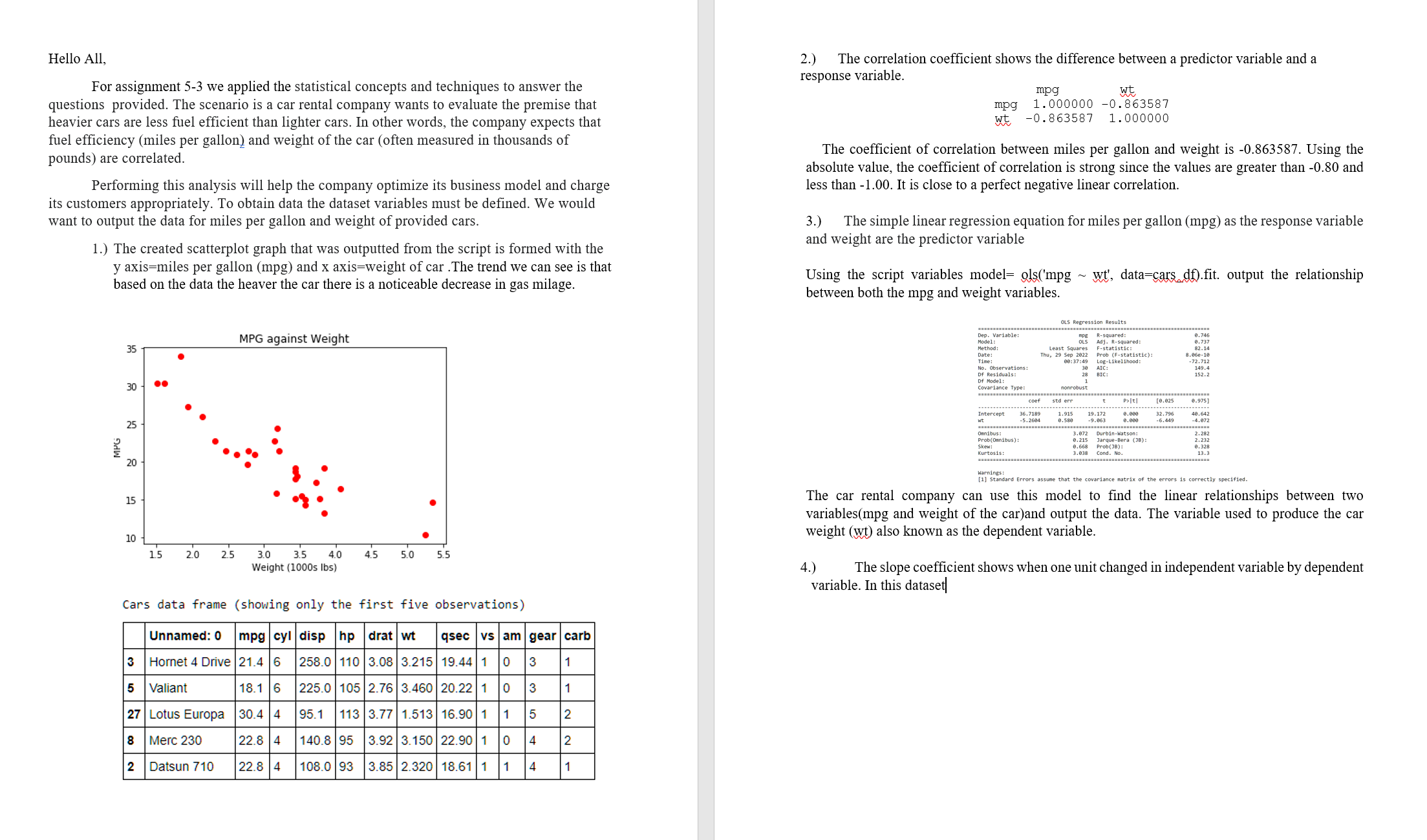
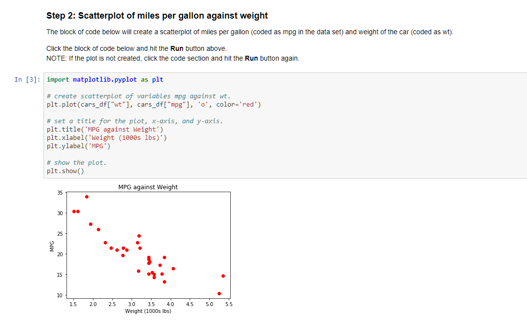
In your initial post, address the following items: 1. You created a scatterplot of miles per gallon against weight; check to make sure it was included in your attachment. Does the graph show any trend? If yes, is the trend what you expected? Why or why not? See Step 2 in the Python script. 2. What is the coefficient of correlation between miles per gallon and weight? What is the sign of the correlation coefficient? Does the coefficient of correlation indicate a strong correlation, weak correlation, or no correlation between the two variables? How do you know? See Step 3 in the Python script. 3. Write the simple linear regression equation for miles per gallon as the response variable and weight as the predictor variable. How might the car rental company use this model? See Step 4 in the Python script. 4. What is the slope coefficient? Is this coefficient significant at a 5% level of significance (alpha=0.05)? (Hint: Check the P-value, pI'ltl, for weight in the Python output.) See Step 4 in the Python script. In [1]: import pandas as pd from IPython . display import display, HTML # read data from mtcars. csv data set. cars_df_orig = pd. read_csv("https://53-us-west-2. amazonaws. com/data-analytics. zybooks.com/mtcars.csv") # randomly pick 30 observations without replacement from mtcars dataset to make the data unique to you. cars_df = cars_df_orig. sample(n=30, replace=False) # print only the first five observations in the data set. print("\ Cars data frame (showing only the first five observations)") display (HTML(cars_df . head() . to_html() ) ) Cars data frame (showing only the first five observations) Unnamed: 0 mpg cyl disp hp drat wt qsec VS am gear carb 3 Hornet 4 Drive 21.4 6 258.0 110 3.08 3.215 19.44 1 0 3 1 5 Valiant 18.1 6 225.0 105 2.76 3.460 20.22 1 0 3 1 27 Lotus Europa 30.4 4 95.1 113 3.77 1.513 16.90 1 1 5 2 8 Merc 230 22.8 4 140.8 95 3.92 3.150 22.90 1 0 4 2 2 Datsun 710 22.8 4 108.0 193 3.85 2.320 18.61 1 4 1Step 2: Scatterplot of miles per gallon against weight The block of code below will create a scatterplot of miles per gallon (coded as mpg in the data set) and weight of the car (coded as wt). Click the block of code below and hit the Run button above. NOTE: If the plot is not created, click the code section and hit the Run button again. In [3]: import matplotlib. pyplot as plt # create scatterplot of variables mpg against wt. plt. plot(cars_df["wt"], cars_df["mpg"], 'o', color='red' ) # set a title for the plot, x-axis, and y-axis. pit. title('MPG against Weight" ) pit. xlabel( Weight (10005 1bs) ' ) plt . ylabel('MPG' ) # show the plot. pit . show ( ) MPG against Weight 35 30 25 . MPG 20 15 10 15 20 2.5 3.0 3.5 4.0 4.5 5.0 5.5 Weight (1000s lbs)In [4]: # create correlation matrix for mpg and wt. # the correlation coefficient between mpg and wt is contained in the cell for mpg row and wt column (or wt row and mpg column) mpg_wt_corr = cars_df[ ['mpg' , 'wt' ]] . corr() print (mpg_wt_corr) mpg wt mpg 1.000000 -0.863587 wt -0.863587 1.090900 Step 4: Simple linear regression model to predict miles per gallon using weight The block of code below produces a simple linear regression model using "miles per gallon" as the response variable and "weight" (of the car) as a predictor variable. The ols method in statsmodels. formula.api submodule returns all statistics for this simple linear regression model. Click the block of code below and hit the Run button above. In [5]: from statsmodels. formula. api import ols # create the simple Linear regression model with mpg as the response variable and weight as the predictor variable model = ols('mpg ~ wt' , data=cars_df) . fit() #print the model summary print (model . summary ( ) ) OLS Regression Results Dep. Variable: mpg R-squared: 0. 746 Model : OLS Adj. R-squared: 0.737 Method: Least Squares F-statistic: 82.14 Date: Thu, 29 Sep 2022 Prob (F-statistic) : 8. 06e-10 Time : 08 : 37:49 Log-Likelihood: -72. 712 No. Observations: 30 AIC : 149.4 Of Residuals : 28 BIC : 152.2 Df Model : 1 Covariance Type: nonrobust coef std err P> t 0. 025 3.975] Intercept 36.7189 1.915 19.172 0.000 32.796 40 . 642 wt -5.2604 0.580 -9.063 3.000 -6.449 -4.072 Omnibus : 3.072 Durbin-Watson: 2. 282 Prob (Omnibus ) : 0. 215 Jarque-Bera (JB) : 2.232 Skew: 0 . 668 Prob( JB) : 0. 328 Kurtosis : 3.038 Cond. No. 13.3 Warnings : [1] Standard Errors assume that the covariance matrix of the errors is correctly specified.Hello All. For assignment 5-3 We applied the statistical concepts and techniques to answer the questions provided. The scenario is a car rental company wants to evaluate the premise that heavier cars are less fuel efficient than lighter cars. In other words. the company expects that fuel efficiency (miles per gallon; and weight of the car (often measured in thousands of pounds) are correlated Performing this analysis will help the company optimize its business model and charge its customers appropriately. To obtain data the dataset variables must be dened. We would want to output the data for miles per gallon and weight of provided cars. 1.) The created scatterplot graph that was outputted from the script is formed with the y axis:miles per gallon (mpg) and x axis:weight of car .The trend we can see is that based on the data the heaver the car there is a noticeable decrease in gas milage. MPG against weight 35 O 30 no 0 O 25 . g 0 O 2 a... o 20 o ' . O O O 15 0'. . I 10 0 1 5 20 25 30 35 so 45 50 55 Welghl noon; lbs] Cars data frame (showing only the first five observations) Unnamedzo mpg cyl disp hp arat wt qsec vs am gear cart) 3 HorneteDnve 214 S 2580 110 308 3215 1944 1 0 3 1 5 Valiant 181 6 225.0 105 2.76 3.460 20.22 1 0 3 1 27 Lotus Europa 304 A 95.1 113 377 1513 1690 1 1 5 2 8 Merc230 228 4 140.8 95 3.92 3.150 22.90 1 0 4 2 2 Datsun710 22B 4 1080 93 385 2320 1861 1 1 4 1 2.) The correlation coefcient shows the difference between a predictor variable and a response variable. mpg at mpg 1.000000 70.863587 at, 70.863587 1.000000 The coefficient of correlation between miles per gallon and weight is -0.863587. Using the absolute value, the coefcient of correlation is strong since the values are greater than -O.80 and less than 1.00. It is close to a perfect negative linear correlation. 3.) The simple linear regression equation for miles per gallon (mpg) as the response variable and weight are the predictor variable Using the script Variables model: glsCmpg ~ m, dathgrsudt. output the relationship between both the mpg and weight variables. on Irirnnm mum um mm ' we tmmm m swim mm mm w me warm. mm a. m gm. is (mum mm The car rental company can use this model to find the linear relationships between two variables(mpg and weight of the car)and output the data. The variable used to produce the car weight (\\vylt) also known as the dependent variable. 4.) The slope coefcient shows when one unit changed in independent variable by dependent variable. In this dataseti