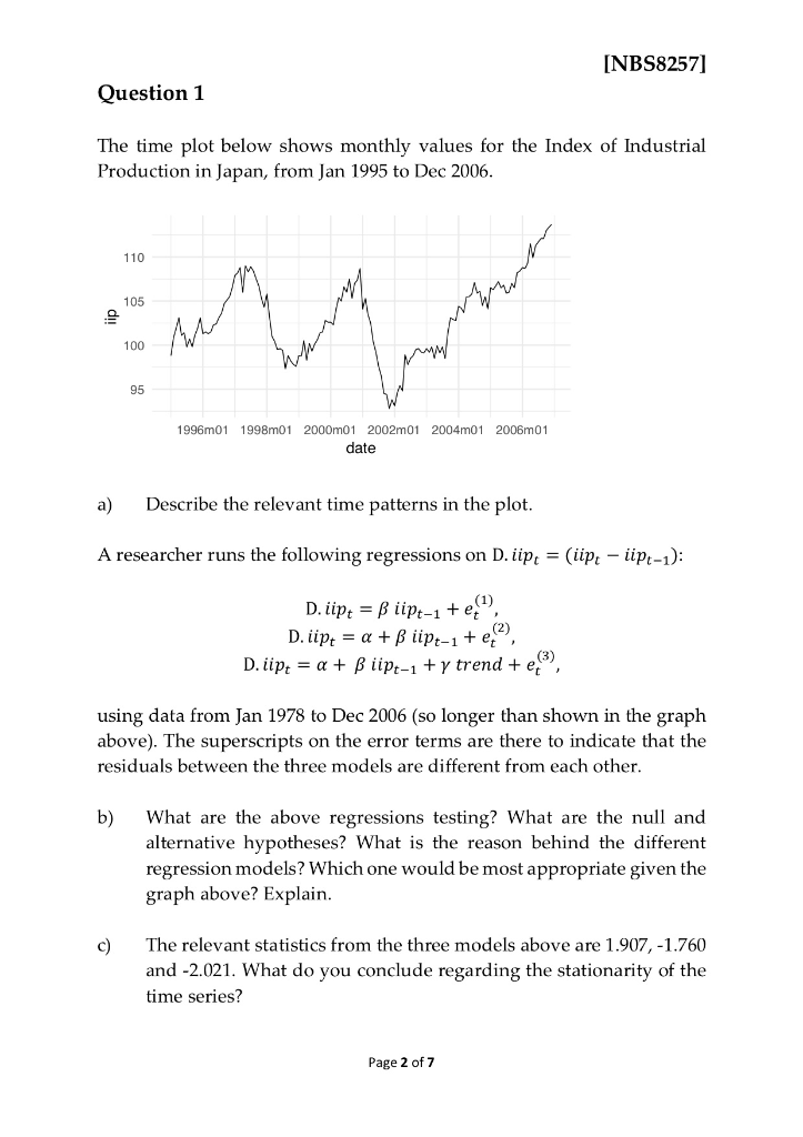
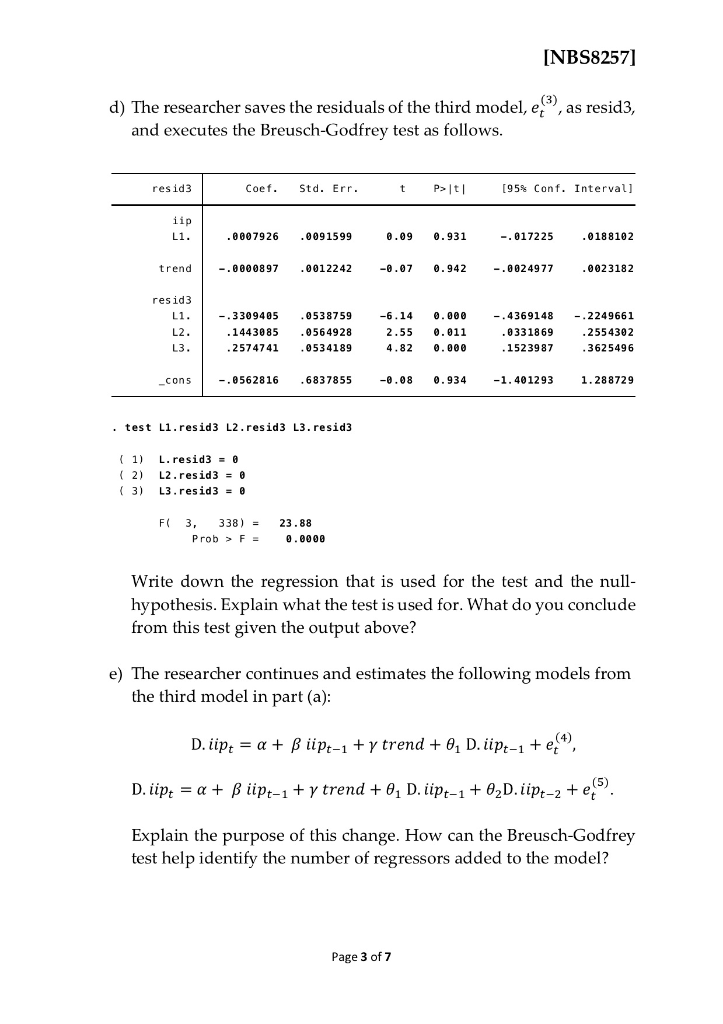
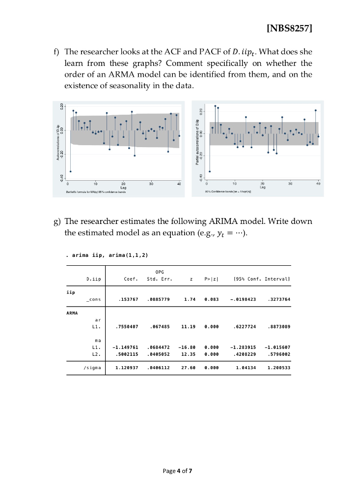
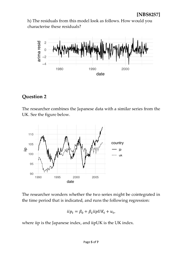
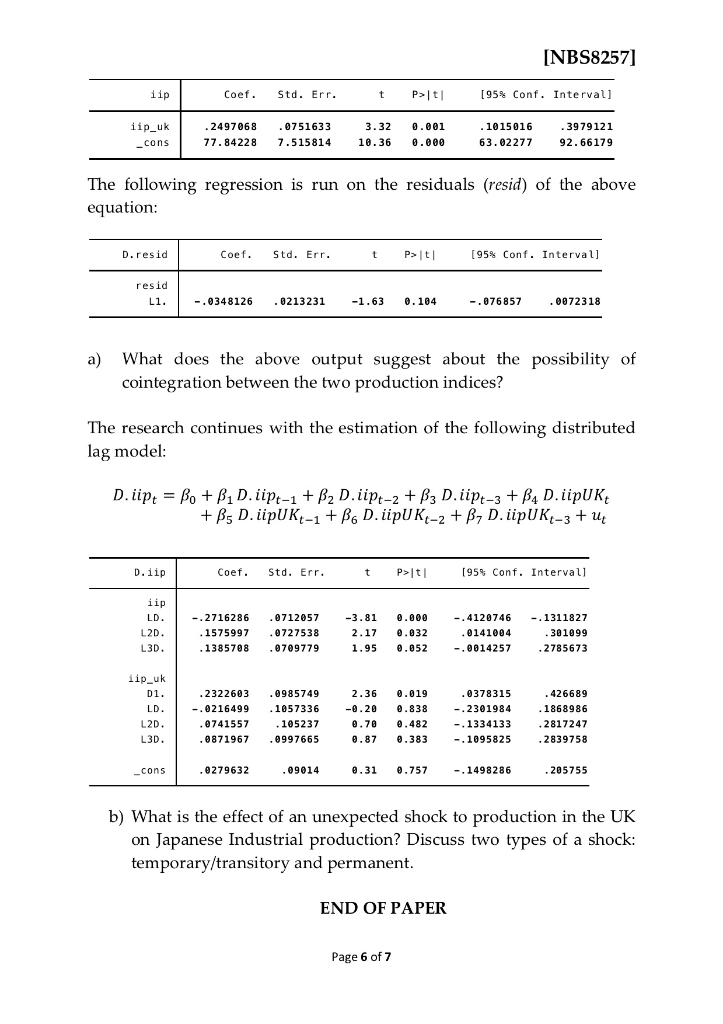
INBS8257] Question 1 The time plot below shows monthly values for the Index of Industrial Production in Japan, from Jan 1995 to Dec 2006 110 105 100 95 1996m01 1998m01 2000m01 2002m01 2004m01 2006m01 date a) Describe the relevant time patterns in the plot A researcher runs the following regressions on D. iipt - (iipt - iipt-1) using data from Jan 1978 to Dec 2006 (so longer than shown in the graph above). The superscripts on the error terms are there to indicate that the residuals between the three models are different from each other b) What are the above regressions testing? What are the null and alternative hypotheses? What is the reason behind the different regression models? Which one would be most appropriate given the graph above? Explairn c) The relevant statistics from the three models above are 1.907, -1.760 and -2.021. What do you conclude regarding the stationarity of the time series? Page 2 of7 INBS8257] d) The researcher saves the residuals of the third model, e as resid3, and executes the Breusch-Godfrey test as follows. resid3 Coef. Std. Err [95% Conf. Interval] iip 0007926 0091599 0.09 0.931 - 017225 0188102 L1. 0023182 trend 00008970012242 -0.07 .942-.0824977 resid3 L1 -.3309405 0538759-6.14 0.900.4369148 - .2249661 L2 1443085 0564928 2.55 0.011 0331869 .2554302 4.82 0.000 L3 2574741 0534189 1523987 3625496 -.0562816 6837855 -0.080.934 -1.401293 1.288729 _cons . test L1.resid3 L2.resid3 L3. resid3 {1) L.resid3= 2) L2.resid30 3) L3.resid30 F 3, 338) 23.88 Prob > F= 0.0000 Write down the regression that is used for the test and the null- hypothesis. Explain what the test is used for. What do you conclude from this test given the output above? e) The researcher continues and estimates the following models from the third model in part (a) Explain the purpose of this change. How can the Breusch-Godfrey test help identify the number of regressors added to the model? Page 3 of7 INBS8257] f) The researcher looks at the ACF and PACF of D. iipt. What does she learn from these graphs? Comment specifically on whether the order of an ARMA model can be identified from them, and on the existence of seasonality in the data Lag Lag g) The researcher estimates the following ARIMA model. Write down the estimated model as an equation (e.g., Vt- ..) . arima iip, arima (1,1,2) OPG D.iip Coef . Std. Err. [95% Conf. Interval] iip 153767 0885779 1.74 0.083-.0198423 3273764 ARMA 6227724 7550407 067485 11.19 0.000 8873089 ma L1. -1.149761 068447216.80 0.000 -1.283915 -1.015607 5002115 0405052 12.35 0.000 4208229 5796082 1.120937 /sigma 046112 27.60 0.00e 1.94134 1.200533 Page 4 of7 INBS8257] h) The residuals from this model look as follows. How would you characterise these residuals? -4 1980 1990 2000 date Question 2 The researcher combines the Japanese data with a similar series from the UK. See the figure below 110 country 105 ip 100 95, 90 1990 1995 2000 2005 date The researcher wonders whether the two series might be cointegrated in the time period that is indicated, and runs the following regression where iip is the Japanese index, and iipUK is the UK index Page 5 of7 INBS8257] iip Coef Std Err [95% Conf. Interval] 0751633 1015816 3979121 iip uk 2497068 3.32 0.001 10.36 0.000 63.02277 92.66179 77.84228 7.515814 -cons The following regression is run on the residuals (resid) of the above equation Coef Std Err [95% Conf. Interval] D.resid resid -.876857 0072318 L1 -.03481268213231-1.63 0.104 a) What does the above output suggest about the possibility of cointegration between the two production indices? The research continues with the estimation of the following distributed lag model D.iip Coef. Std. Err. [95% Conf. Interval] iip -2716286.0712057-3.81 0.0004120746 .1311827 2.17 .032 381099 L2D 1575997 0727538 0141004 L3D 1385708 0709779 1.95 0.852 -.0014257 2785673 iip_uk 0378315 426689 .2322603 0985749 2.36 0.019 -.02164991057336 -0.20 0.838.2301984 1868986 L2D 105237 8.70 e,482 0741557 -.1334133 2817247 L3D 9871967 0997665 0.87 0.383 2839758 -.1095825 09014 0279632 8.31 .757 205755 -.1498286 -cons b) What is the effect of an unexpected shock to production in the UK on Japanese Industrial production? Discuss two types of a shock: temporary/transitory and permanent END OF PAPER Page 6 of7 INBS8257] Question 1 The time plot below shows monthly values for the Index of Industrial Production in Japan, from Jan 1995 to Dec 2006 110 105 100 95 1996m01 1998m01 2000m01 2002m01 2004m01 2006m01 date a) Describe the relevant time patterns in the plot A researcher runs the following regressions on D. iipt - (iipt - iipt-1) using data from Jan 1978 to Dec 2006 (so longer than shown in the graph above). The superscripts on the error terms are there to indicate that the residuals between the three models are different from each other b) What are the above regressions testing? What are the null and alternative hypotheses? What is the reason behind the different regression models? Which one would be most appropriate given the graph above? Explairn c) The relevant statistics from the three models above are 1.907, -1.760 and -2.021. What do you conclude regarding the stationarity of the time series? Page 2 of7 INBS8257] d) The researcher saves the residuals of the third model, e as resid3, and executes the Breusch-Godfrey test as follows. resid3 Coef. Std. Err [95% Conf. Interval] iip 0007926 0091599 0.09 0.931 - 017225 0188102 L1. 0023182 trend 00008970012242 -0.07 .942-.0824977 resid3 L1 -.3309405 0538759-6.14 0.900.4369148 - .2249661 L2 1443085 0564928 2.55 0.011 0331869 .2554302 4.82 0.000 L3 2574741 0534189 1523987 3625496 -.0562816 6837855 -0.080.934 -1.401293 1.288729 _cons . test L1.resid3 L2.resid3 L3. resid3 {1) L.resid3= 2) L2.resid30 3) L3.resid30 F 3, 338) 23.88 Prob > F= 0.0000 Write down the regression that is used for the test and the null- hypothesis. Explain what the test is used for. What do you conclude from this test given the output above? e) The researcher continues and estimates the following models from the third model in part (a) Explain the purpose of this change. How can the Breusch-Godfrey test help identify the number of regressors added to the model? Page 3 of7 INBS8257] f) The researcher looks at the ACF and PACF of D. iipt. What does she learn from these graphs? Comment specifically on whether the order of an ARMA model can be identified from them, and on the existence of seasonality in the data Lag Lag g) The researcher estimates the following ARIMA model. Write down the estimated model as an equation (e.g., Vt- ..) . arima iip, arima (1,1,2) OPG D.iip Coef . Std. Err. [95% Conf. Interval] iip 153767 0885779 1.74 0.083-.0198423 3273764 ARMA 6227724 7550407 067485 11.19 0.000 8873089 ma L1. -1.149761 068447216.80 0.000 -1.283915 -1.015607 5002115 0405052 12.35 0.000 4208229 5796082 1.120937 /sigma 046112 27.60 0.00e 1.94134 1.200533 Page 4 of7 INBS8257] h) The residuals from this model look as follows. How would you characterise these residuals? -4 1980 1990 2000 date Question 2 The researcher combines the Japanese data with a similar series from the UK. See the figure below 110 country 105 ip 100 95, 90 1990 1995 2000 2005 date The researcher wonders whether the two series might be cointegrated in the time period that is indicated, and runs the following regression where iip is the Japanese index, and iipUK is the UK index Page 5 of7 INBS8257] iip Coef Std Err [95% Conf. Interval] 0751633 1015816 3979121 iip uk 2497068 3.32 0.001 10.36 0.000 63.02277 92.66179 77.84228 7.515814 -cons The following regression is run on the residuals (resid) of the above equation Coef Std Err [95% Conf. Interval] D.resid resid -.876857 0072318 L1 -.03481268213231-1.63 0.104 a) What does the above output suggest about the possibility of cointegration between the two production indices? The research continues with the estimation of the following distributed lag model D.iip Coef. Std. Err. [95% Conf. Interval] iip -2716286.0712057-3.81 0.0004120746 .1311827 2.17 .032 381099 L2D 1575997 0727538 0141004 L3D 1385708 0709779 1.95 0.852 -.0014257 2785673 iip_uk 0378315 426689 .2322603 0985749 2.36 0.019 -.02164991057336 -0.20 0.838.2301984 1868986 L2D 105237 8.70 e,482 0741557 -.1334133 2817247 L3D 9871967 0997665 0.87 0.383 2839758 -.1095825 09014 0279632 8.31 .757 205755 -.1498286 -cons b) What is the effect of an unexpected shock to production in the UK on Japanese Industrial production? Discuss two types of a shock: temporary/transitory and permanent END OF PAPER Page 6 of7