Indah conducted an experiment to determine the effects of professor (Prof. Halgren, an indifferent professor who didn't care about student achievement; Prof. Wurmkiln, a harsh professor who punished students with draconian zeal for mild errors; and Prof. Baxter, widely renowned as a charming, witty, funny professor with much compassion his students and interest in their progress) and time (Time 1, beginning of the semester; Time 2, middle of the semester; and Time 3, end of the semester) had an impact on students' confidence in their statistics competency [1(no confidence at all) to 10(considers oneself a genius in statistics)]. They gathered data from 30 participants, 10 from each class, and measured their participants' statistics confidence at three time points across the semester. Indah then conducted a 3x3 mixed factorial ANOVA on her data. Below are the results of their analysis:

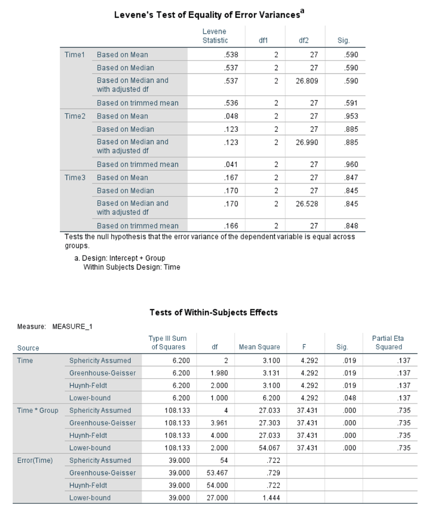
How do you know if the assumption of homogeneity of variance for each level of Time been violated or met? How do you determine such?

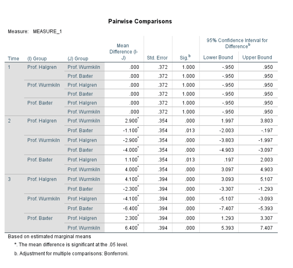
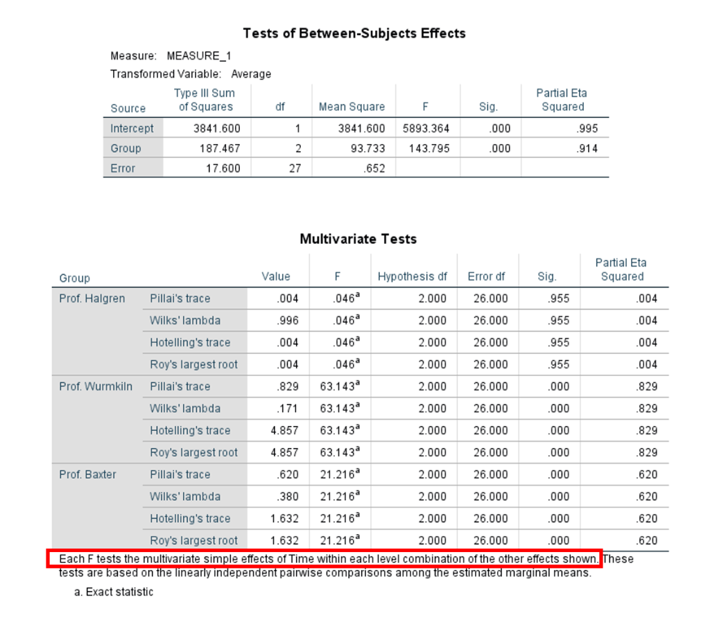
Which simple effect(s) is/are non-significant?

What would a full results report for Indah's findings look like?

Levene's Test of Equality of Error Variances Levene Statistic df1 df2 Sig Time1 Based on Mean .538 2 27 590 Based on Median .537 2 27 590 Based on Median and 537 26.809 590 with adjusted df Based on trimmed mean 536 NJ 27 .591 Time2 Based on Mean 048 27 953 Based on Median 123 27 885 Based on Median and 123 26.990 885 with adjusted df Based on trimmed mean 041 2 27 960 Time3 Based on Mean 167 2 27 .847 Based on Median 170 27 845 Based on Median and 170 26.528 845 with adjusted df Based on trimmed mean .166 2 27 .848 Tests the null hypothesis that the error variance of the dependent variable is equal across groups. a. Design: Intercept + Group Within Subjects Design: Time Tests of Within-Subjects Effects Measure: MEASURE_1 Type Ill Sum Partial Eta Source of Squares df Mean Square F Sig Squared Time Sphericity Assumed 6.200 2 3.100 4.292 19 137 Greenhouse-Geisser 6.200 1.980 3.131 4.292 .019 137 Huynh-Feldt 6.200 2.000 3.100 4.292 019 137 Lower-bound 6.200 1.000 6.200 4.292 048 137 Time * Group Sphericity Assumed 108.133 27.033 37.431 000 735 Greenhouse-Geisser 108.133 3.961 27.303 37.431 000 735 Huynh-Feldt 108.133 4.000 27.033 37.431 .000 .735 Lower-bound 108.133 2.000 54.067 37.431 000 .735 Error(Time) Sphericity Assumed 39.000 54 722 Greenhouse-Geisser 39.000 53.467 .729 Huynh-Feldt 39.000 54.000 722 Lower-bound 39.000 27.000 1.444Pairwise Comparisons Measure: MEASURE_1 95% Confidence Interval for Mean Difference Difference (1- Time (1) Group (J) Group J ) Std. Error Sig b Lower Bound Upper Bound Prof. Halgren Prof. Wurmkiln 000 372 1.000 .950 950 Prof. Baxter 000 372 1.000 .950 950 Prof. Wurmkiln Prof. Halgren 000 .372 1.000 -.950 950 Prof. Baxter 000 372 1.000 .950 950 Prof. Baxter Prof. Halgren 000 372 1.000 .950 950 Prof. Wurmkiln 000 372 1.000 -.950 950 2 Prof. Halgren Prof. Wurmkiln 2.900 354 000 1.997 3.803 Prof. Baxter -1.100 .354 013 2.003 -.197 Prof. Wurmkiln Prof. Halgren -2.900 354 000 -3.803 -1.997 Prof. Baxter -4.000 354 000 -4.903 -3.097 Prof. Baxter Prof. Halgren 1.100 354 013 197 2.003 Prof. Wurmkiln 4.000 .354 000 3.097 4.903 3 Prof. Halgren Prof. Wurmkiln 4.100 .394 000 3.093 5.107 Prof. Baxter -2.300 .394 000 3.307 -1.293 Prof. Wurmkiln Prof. Halgren -4.100 394 000 -5.107 -3.093 Prof. Baxter -6.400 .394 000 7.407 -5.393 Prof. Baxter Prof. Halgren 2.300 .394 000 1.293 3.307 Prof. Wurmkiln 6.400 394 000 5.393 7.407 Based on estimated marginal means *. The mean difference is significant at the .05 level. b. Adjustment for multiple comparisons: Bonferroni.Tests of Between-Subjects Effects Measure: MEASURE_1 Transformed Variable: Average Type Ill Sum Partial Eta Source of Squares df Mean Square F Sig. Squared Intercept 3841.600 1 3841.600 5893.364 000 995 Group 187.467 2 93.733 143.795 000 914 Error 17.600 27 652 Multivariate Tests Partial Eta Group Value F Hypothesis of Error of Sig. Squared Prof. Halgren Pillai's trace .004 046 2.000 26.000 955 004 Wilks' lambda .996 046 2.000 26.000 955 004 Hotelling's trace 004 046 2.000 26.000 955 004 Roy's largest root 004 046a 2.000 26.000 955 .004 Prof. Wurmkiln Pillai's trace 829 63.143 2.000 26.000 000 829 Wilks' lambda 171 63.1432 2.000 26.000 000 829 Hotelling's trace 4.857 63.143 2.000 26.000 000 829 Roy's largest root 4.857 63.143 2.000 26.000 000 829 Prof. Baxter Pillai's trace 620 21.216 2.000 26.000 000 620 Wilks' lambda 380 21.216 2.000 26.000 000 620 Hotelling's trace 1.632 21.216 2.000 26.000 000 .620 Roy's largest root 1.632 21.216 2.000 26.000 .000 620 Each F tests the multivariate simple effects of Time within each level combination of the other effects shown. These tests are based on the linearly independent pairwise comparisons among the estimated marginal means a. Exact statisticPairwise Comparisons Measure: MEASURE_1 95% Confidence Interval for Mean Difference Difference (1- Group (1) Time (J) Time J) Std. Error Sig. b Lower Bound Upper Bound Prof. Halgren 1 2 000 384 1,000 .980 980 3 ..100 362 1.000 -1.023 823 2 1 .000 .384 1.000 .980 980 w ..100 394 1.000 -1.106 906 3 100 362 1.000 -.823 1.023 NN - 100 .394 1.000 -.906 1.106 Prof. Wurmkiln 1 2.900 .384 000 1.920 3.880 3 4.000 .362 .000 3.077 4.923 2 -2.900 .384 000 3.880 -1.920 3 1.100 .394 028 .094 2.106 3 -4.000 .362 000 4.923 -3.077 N -1.100 .394 028 2.106 .094 Prof. Baxter 1 N -1.100 384 024 -2.080 .120 3 -2.400 362 000 -3.323 -1.477 2 1.100 384 024 120 2.080 3 -1.300 394 008 -2.306 .294 3 2.400 362 000 1.477 3.323 1.300 394 008 294 2.306 Based on estimated marginal means *. The mean difference is significant at the .05 level. b. Adjustment for multiple comparisons: Bonferroni. Univariate Tests Measure: MEASURE_1 Sum of Partial Eta Time Squares dif Mean Square F Sig. Squared Contrast .000 2 .000 000 1.000 .000 Error 18.700 27 693 2 Contrast 85.400 2 42.700 68.219 .000 835 Error 16.900 27 626 Contrast 210.200 2 105.100 135.129 000 909 Error 21.000 27 778 Each F tests the simple effects of Group within each level combination of the other effects shown. These tests are based on the linearly independent pairwise comparisons among the estimated marginal means.Descriptive Statistics Group Mean Std. Deviation N Time1 Prof. Halgren 6.9000 87560 10 Prof. Wurmkiln 6.9000 87560 10 Prof. Baxter 6.9000 73786 10 Total 6.9000 80301 30 Time2 Prof. Halgren 6.9000 .73786 10 Prof. Wurmkiln 4.0000 .81650 10 Prof. Baxter 8.0000 81650 10 Total 6.3000 1.87819 30 Time 3 Prof. Halgren 7.0000 94281 10 Prof. Wurmkiln 2.9000 87560 10 Prof. Baxter 9.3000 82327 10 Total 6.4000 2.82355 30 Mauchly's Test of Sphericity Measure: MEASURE_1 Epsilonb Approx. Chi- Greenhouse- Within Subjects Effect Mauchly's W Square df Sig. Geisser Huynh-Feldt Lower-bound Time 990 .260 2 878 990 1.000 .500 Tests the null hypothesis that the error covariance matrix of the orthonormalized transformed dependent variables is proportional to an identity matrix. a. Design: Intercept + Group Within Subjects Design: Time b. May be used to adjust the degrees of freedom for the averaged tests of significance. Corrected tests are displayed in the Tests of Within-Subjects Effects table