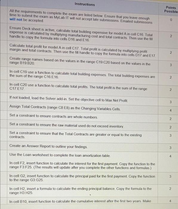
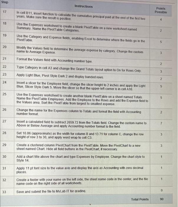
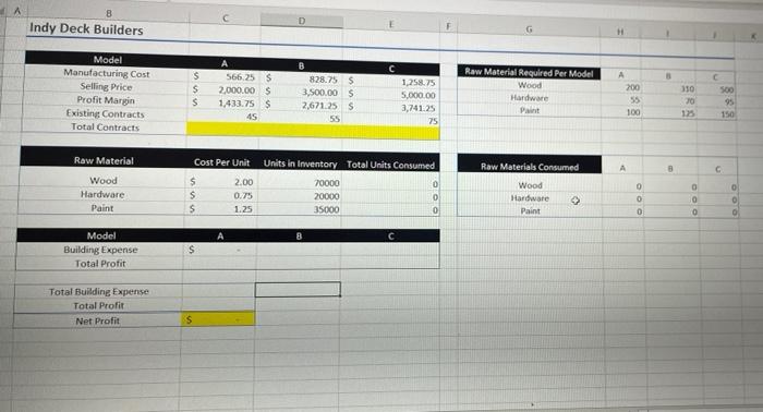
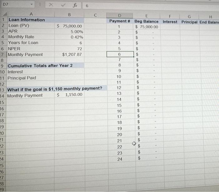
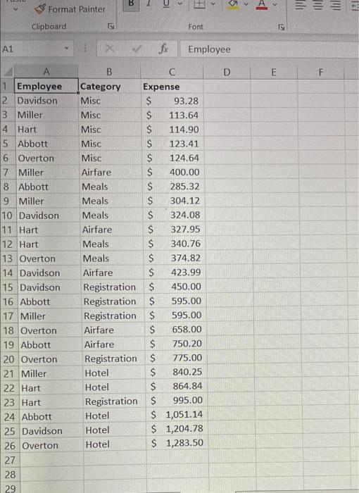
Instructions Points Possible 0 2 All the requirements to complete the exam are listed below. Ensure that you leave enough time to submit the exam as Myl.ab It will not accept late submissions. Emailed submissions will not be accepted Ensure Deck sheet is active, calculate total building expensive for model Ain cell C16 Total expense is calculated by multiplying manufacturing cost and total contracts. Then use the fill handle to copy the formula into cells D16 and E16. Calculate total profit for model A in cell C17 Total profit is calculated by multiplying profit margin and total contracts Then use the fill handle to copy the formula into cells D17 and E17 Create range names based on the values in the range C19 C20 based on the values in the range B19 B20 In cell C19 use a function to calculate total building expenses. The total building expenses are the sum of the range C16 E 16. In cell C20 use a function to calculate total profits. The total profit is the sum of the range C17 E17 2 3 2. 2 2 If not loaded, load the Solver add-in. Set the objective cell to Max Net Profit Assign Total Contracts (range C8E8) as the Changing Variables Cells 3 4 Set a constraint to ensure contracts are whole numbers 2 2 3 3 4 Set a constraint to ensure the raw material used do not exceed inventory Set a constraint to ensure that the Total Contracts are greater or equal to the existing contracts Create an Answer Report to outline your findings. Use the Loan worksheet to complete the loan amortization table. In cell F2, insert function to calculate the interest for the first payment. Copy the function to the range F3 F25. (The results will update after you complete the other functions and formulas.) In cell G2, insert function to calculate the principal paid for the first payment. Copy the function to the range G3 G25 In cell H2, insert a formula to calculate the ending principal balance Copy the formula to the range H3 H25 In cell B10, insert function to calculate the cumulative interest after the first two years Make 3 2. 4 Step Instructions 17 Points Possible In cell B11, insert function to calculate the cumulative principal paid at the end of the first two years. Make sure the result is positive 4 18 Use the Expenses worksheet to create a blank PivotTable on a new worksheet named Summary. Name the PivotTable Categories 2 19 Use the Category and Expense fields, enabling Excel to determine where the fields go in the Pivot Table 5 20 Modify the Values field to determine the average expense by category. Change the custom name to Average Expense. 3 21 Format the Values field with Accounting number type 2 22 Type Category in cell A3 and change the Grand Totals layout option to On for Rows Only 3 23 2 24 Apply Light Blue, Pivot Style Dark 2 and display banded rows Insert a slicer for the Employee field, change the slicer height to 2 inches and apply the Light Blue, Slicer Style Dark 5. Move the slicer so that the upper-left corner is in cell A10 5 25 5 26 2 27 7 28 3 3 Use the Expenses worksheet to create another blank PivotTable on a sheet named Totals Name the PivotTable Employees. Add the Employee to the Rows and add the Expense field to the Values area. Sort the PivotTable from largest to smallest expense Change the name for the Expenses column to Totals and format the field with Accounting number format Insert a calculated field to subtract 2659.72 from the Totals field. Change the custom name to Above or Below Average and apply Accounting number format to the field. Set 10.86 (approximate) as the width for column B and 13.71 for column C change the row height of row 3 to 30, and apply word wrap to cell C3 Create a clustered column PivotChart from the Pivottable. Move the PivotChart to a new sheet named Chart. Hide all field buttons in the PivotChart if necessary. Add a chart title above the chart and type Expenses by Employee. Change the chart style to Style 14 Apply 11 pt font size to the value axis and display the axis as Accounting with zero decimal places Create a footer with your name on the left side, the sheet name code in the center and the file name code on the right side of all worksheets. 29 3 30 1 31 1 32 1 33 Save and submit the file to MyLab IT for grading Total Points 90 A D Indy Deck Builders C Model Manufacturing Cost Selling Price Profit Margin Existing Contracts Total Contracts $ s S 566,25 $ 2,000.00 $ 1.433.75$ 45 B 828.75 S 3,500.00 5 2,671.255 55 1,258.75 5,000.00 3,741.25 75 Raw Material Required Per Model Wood Hardware Paint A 200 55 100 310 30 125 C 500 95 150 Raw Material Cost Per Unit Raw Materials Consumed A C Us Wood Hardware Paint Units in Inventory Total Units Consumed 70000 0 20000 O 35000 0 2.00 0.75 1.25 $ $ Wood Hardware Paint o 0 0 > 0 0 Model Building Expense Total Profit $ Total Building Expense Total Profit Net Profit S D7 fo 6 G H Interest Principal End Balanc D E Payment # Beg Balance $ 75,000.00 2 $ $ 4 5 $ 1 $ 7 8 9 COVOAN B 1 Loan Information 2 Loan (PV) $ 75,000.00 3 APR 5.00% 4 Monthly Rate 0.42% 5 Years for Loan 6 6 NPER 72 7 Monthly Payment $1,207.87 8 9 Cumulative Totals after Year 2 10 Interest 11 Principal Paid 12 73 What if the goal is $1,150 monthly payment? 74 Monthly Payment $ 1,150.00 15 16 17 18 19 20 21 22 10 11 12 13 14 * - * - * - 0 - - 15 16 17 18 19 20 21 22 23 24 $ $ $ $ $ $ $ $ $ $ - + 3 24 25 26 27 28 29 U TU IM * Format Painter Clipboard 2 Font 2 A1 f Employee D E 1 Employee 2 Davidson 3 Miller 4 Hart 5 Abbott 6 Overton 7 Miller 8 Abbott 9 Miller 10 Davidson 11 Hart 12 Hart 13 Overton 14 Davidson 15 Davidson 16 Abbott 17 Miller 18 Overton 19 Abbott 20 Overton 21 Miller 22 Hart 23 Hart 24 Abbott 25 Davidson 26 Overton 27 28 B C Category Expense Misc $ 93.28 Misc S 113.64 Misc $ 114.90 Misc 123.41 Misc $ 124.64 Airfare $ 400.00 Meals $ 285.32 Meals $ 304.12 Meals $ 324.08 Airfare $ 327.95 Meals $ 340.76 Meals $ 374.82 Airfare $ 423.99 Registration $ 450.00 Registration S 595.00 Registration $ 595.00 Airfare $ 658.00 Airfare $ 750.20 Registration $ 775.00 Hotel $ 840.25 Hotel $ 864.84 Registration $ 995.00 Hotel $ 1,051.14 Hotel $ 1,204.78 Hotel $ 1,283.50 29 Instructions Points Possible 0 2 All the requirements to complete the exam are listed below. Ensure that you leave enough time to submit the exam as Myl.ab It will not accept late submissions. Emailed submissions will not be accepted Ensure Deck sheet is active, calculate total building expensive for model Ain cell C16 Total expense is calculated by multiplying manufacturing cost and total contracts. Then use the fill handle to copy the formula into cells D16 and E16. Calculate total profit for model A in cell C17 Total profit is calculated by multiplying profit margin and total contracts Then use the fill handle to copy the formula into cells D17 and E17 Create range names based on the values in the range C19 C20 based on the values in the range B19 B20 In cell C19 use a function to calculate total building expenses. The total building expenses are the sum of the range C16 E 16. In cell C20 use a function to calculate total profits. The total profit is the sum of the range C17 E17 2 3 2. 2 2 If not loaded, load the Solver add-in. Set the objective cell to Max Net Profit Assign Total Contracts (range C8E8) as the Changing Variables Cells 3 4 Set a constraint to ensure contracts are whole numbers 2 2 3 3 4 Set a constraint to ensure the raw material used do not exceed inventory Set a constraint to ensure that the Total Contracts are greater or equal to the existing contracts Create an Answer Report to outline your findings. Use the Loan worksheet to complete the loan amortization table. In cell F2, insert function to calculate the interest for the first payment. Copy the function to the range F3 F25. (The results will update after you complete the other functions and formulas.) In cell G2, insert function to calculate the principal paid for the first payment. Copy the function to the range G3 G25 In cell H2, insert a formula to calculate the ending principal balance Copy the formula to the range H3 H25 In cell B10, insert function to calculate the cumulative interest after the first two years Make 3 2. 4 Step Instructions 17 Points Possible In cell B11, insert function to calculate the cumulative principal paid at the end of the first two years. Make sure the result is positive 4 18 Use the Expenses worksheet to create a blank PivotTable on a new worksheet named Summary. Name the PivotTable Categories 2 19 Use the Category and Expense fields, enabling Excel to determine where the fields go in the Pivot Table 5 20 Modify the Values field to determine the average expense by category. Change the custom name to Average Expense. 3 21 Format the Values field with Accounting number type 2 22 Type Category in cell A3 and change the Grand Totals layout option to On for Rows Only 3 23 2 24 Apply Light Blue, Pivot Style Dark 2 and display banded rows Insert a slicer for the Employee field, change the slicer height to 2 inches and apply the Light Blue, Slicer Style Dark 5. Move the slicer so that the upper-left corner is in cell A10 5 25 5 26 2 27 7 28 3 3 Use the Expenses worksheet to create another blank PivotTable on a sheet named Totals Name the PivotTable Employees. Add the Employee to the Rows and add the Expense field to the Values area. Sort the PivotTable from largest to smallest expense Change the name for the Expenses column to Totals and format the field with Accounting number format Insert a calculated field to subtract 2659.72 from the Totals field. Change the custom name to Above or Below Average and apply Accounting number format to the field. Set 10.86 (approximate) as the width for column B and 13.71 for column C change the row height of row 3 to 30, and apply word wrap to cell C3 Create a clustered column PivotChart from the Pivottable. Move the PivotChart to a new sheet named Chart. Hide all field buttons in the PivotChart if necessary. Add a chart title above the chart and type Expenses by Employee. Change the chart style to Style 14 Apply 11 pt font size to the value axis and display the axis as Accounting with zero decimal places Create a footer with your name on the left side, the sheet name code in the center and the file name code on the right side of all worksheets. 29 3 30 1 31 1 32 1 33 Save and submit the file to MyLab IT for grading Total Points 90 A D Indy Deck Builders C Model Manufacturing Cost Selling Price Profit Margin Existing Contracts Total Contracts $ s S 566,25 $ 2,000.00 $ 1.433.75$ 45 B 828.75 S 3,500.00 5 2,671.255 55 1,258.75 5,000.00 3,741.25 75 Raw Material Required Per Model Wood Hardware Paint A 200 55 100 310 30 125 C 500 95 150 Raw Material Cost Per Unit Raw Materials Consumed A C Us Wood Hardware Paint Units in Inventory Total Units Consumed 70000 0 20000 O 35000 0 2.00 0.75 1.25 $ $ Wood Hardware Paint o 0 0 > 0 0 Model Building Expense Total Profit $ Total Building Expense Total Profit Net Profit S D7 fo 6 G H Interest Principal End Balanc D E Payment # Beg Balance $ 75,000.00 2 $ $ 4 5 $ 1 $ 7 8 9 COVOAN B 1 Loan Information 2 Loan (PV) $ 75,000.00 3 APR 5.00% 4 Monthly Rate 0.42% 5 Years for Loan 6 6 NPER 72 7 Monthly Payment $1,207.87 8 9 Cumulative Totals after Year 2 10 Interest 11 Principal Paid 12 73 What if the goal is $1,150 monthly payment? 74 Monthly Payment $ 1,150.00 15 16 17 18 19 20 21 22 10 11 12 13 14 * - * - * - 0 - - 15 16 17 18 19 20 21 22 23 24 $ $ $ $ $ $ $ $ $ $ - + 3 24 25 26 27 28 29 U TU IM * Format Painter Clipboard 2 Font 2 A1 f Employee D E 1 Employee 2 Davidson 3 Miller 4 Hart 5 Abbott 6 Overton 7 Miller 8 Abbott 9 Miller 10 Davidson 11 Hart 12 Hart 13 Overton 14 Davidson 15 Davidson 16 Abbott 17 Miller 18 Overton 19 Abbott 20 Overton 21 Miller 22 Hart 23 Hart 24 Abbott 25 Davidson 26 Overton 27 28 B C Category Expense Misc $ 93.28 Misc S 113.64 Misc $ 114.90 Misc 123.41 Misc $ 124.64 Airfare $ 400.00 Meals $ 285.32 Meals $ 304.12 Meals $ 324.08 Airfare $ 327.95 Meals $ 340.76 Meals $ 374.82 Airfare $ 423.99 Registration $ 450.00 Registration S 595.00 Registration $ 595.00 Airfare $ 658.00 Airfare $ 750.20 Registration $ 775.00 Hotel $ 840.25 Hotel $ 864.84 Registration $ 995.00 Hotel $ 1,051.14 Hotel $ 1,204.78 Hotel $ 1,283.50 29